- The battle for Rust Belt Catholicism Charles McElwee, City Journal
- The artwork of Joan Miró Tim Smith-Laing, 1843
- Interpreting Modern Monetary Theory Jeffrey Rogers Hummel, Econlib
- “the most productive in generating cognitive skill” Caetano, Kinsler & Tang, JAE
modern monetary theory
On Scottish Free Banking (a Canadian Perspective)
Yesterday, George Selgin responded on Alt-M to a series of (relatively) recent paper that posit the impossibility of private money. While Selgin does criticize the theoretical reasoning of the papers, the majority of his case is based on the historical experience of private money – notably the Scottish experience with free banking.
I wanted to write something on this, but Selgin got there faster. Indeed, the historical evidence of free banking in Canada, Scotland, Sweden and the limited experiences observed in France and elsewhere provide a strong backing for soundness of private money. Selgin is right to emphasize this.
However, I can provide a small piece of evidence to support his case. It is not only scholars like Selgin who believe that the historical experience of Scotland was positive. As far back as 1835 and as far away as Canada, the robustness of the Scottish free banking experience was lauded. Consider the following quote from a report to the House of Assembly of Upper Canada (modern day Ontario):
“In Scotland, private banking has long existed and fewer failures have occurred there than in any other part of the world; their Joint Stock Banking Companies embrace some of the following principles by which the public are quite secured and the institutions useful as Banks of Deposit and circulation, while the stock is above par, and proved to be a good investment”
This report was actually presented in Canada arguing that Scottish free banking was a solution to a longstanding problem in the colony : dearth of small denominations. The “big problem of small change” was a real issue in the colony and created important frictions. The problem was most likely created by the fixing of exchange rates between the different currencies at levels dissonant with the actual value of different currencies so that “bad money drove out good money” (see Angela Redish’s work). The report recommended legislative actions to encourage the formation of banks that would issue private notes to solve this problem. Newspapers in the neighboring colony of Lower Canada also praised (in the early 1830s) the role that banks played in easing the problem of “poor money”.
I have made an initial foray on this with Mathieu Bédard of Aix-Marseille School of Economics (and we plan to make another few) and showed that the role of free banking in improving economic growth was considerable exactly because of the issue of private money. While Canada is a small, it provides some additional support to the claim that private money can indeed exist, survive and be superior to state money.
Source: House of Assembly of Upper Canada. 1835. Report of the Select Committee to which was referred the subject of The Currency. Toronto : M.Reynolds Printer.
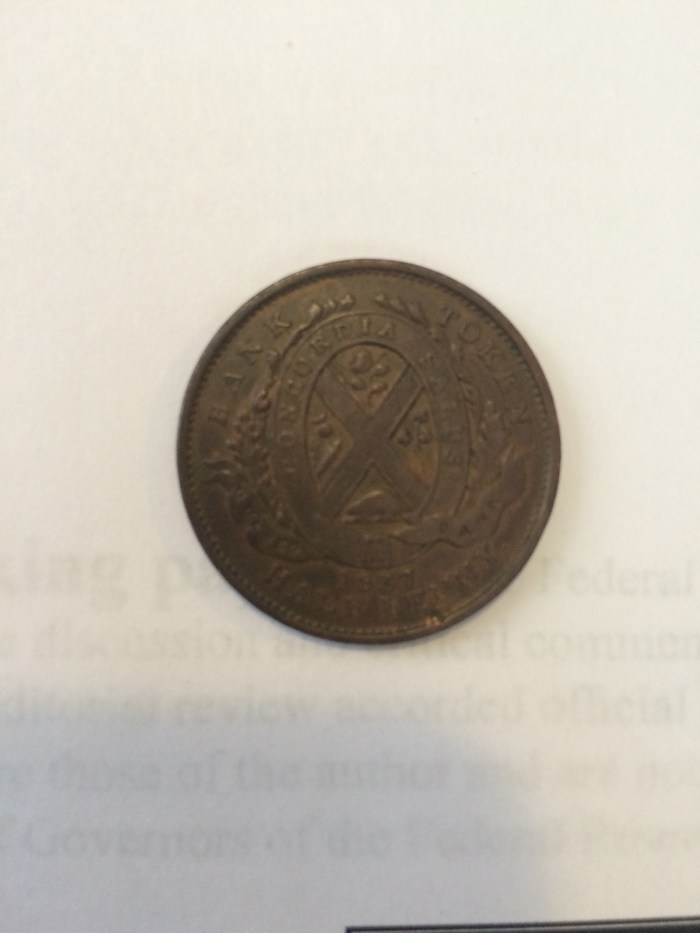
P.S. Below there is a picture of a half-penny issued by the Quebec Bank in 1837 showing that there was even private coinage in Canada.
NGO v. NGDP: In reply to Nunes and Sumner
A week ago, I initiated a discussion on using another indicator of nominal spending instead of NGDP when the time comes to set monetary policy. My claim was that NGDP includes only final goods and as a result, it misses numerous business-to-business transactions. This means that NGDP would not be the best indicator. I propose a shift to a measure that would capture some intermediate transactions.
The result was a response by Nick Rowe (to which I did respond), Matt Rognlie, Marcus Nunes and Scott Sumner (to whom I am responding now). Nunes and Sumner are particularly skeptical of my claim. I am providing a first response here (and I am attempting to expand it for a working paper).
The case against NGDP
GDP has important shortcomings. First of all, thanks to the work of Prescott and McGrattan (2012 : 115-154), we know that a sizable part of capital goods acquisition fails to be included inside GDP. That sizable part is “intangible capital” which Prescott and McGrattan define as the “accumulated know-how from investing in research and development, brands, and organizations which is the most part expensed rather than capitalized” (p.116). Yet, investments in research and development are – in pure theoretical terms – like the acquisition of capital goods. However, national accounts exclude those. Once they’re included in papers like those of Prescott and McGrattan and those of Corrado, Hulten and Sichel (2009), increases in productivity were faster prior to 2008 and that the collapse after 2008 was much more pronounced. In addition, this form of capital is increasing much faster than tangible so that its share of the total capital stock increases. Thus, the error of not capturing this form of capital good investment is actually growing over time causing us to miss both the level and the trend.
A second shortcoming of importance is the role of time in production. Now, just the utterance of these words makes me sound like an Austrian. Yet, this point is very neoclassical since it relies on the time to build approach. In the time-to-build model of the real business cycle approach, production occurs over many periods. Thus changes in monetary policy may have some persistence. The time-to-build model proposes that firms undertake long projects and consume more inputs. In terms of overall transactions, this will mean more and more business to business (B2B) transactions. Hence if an easy monetary policy is inciting individuals to expand their number of projects that have more distant maturities, then a focus on GDP won’t capture the distortionary effects of that policy through. Similarly, if monetary policy tightens (either directly as a fall of the money supply or through an uncompensated change in velocity), the drop in economic activity as projects are closed down will not equally well captured. While this point was initially advanced by Kyland and Prescott (1982), some Austrians economists have taken up the issue (Montgomery 1995a; 1995b; 2006; Wainhouse 1984; Mulligan 2010), several neoclassicals have also taken it up (Kühn 2007; Kalouptsidi 2014; Kyland, Rupert, Sustek, 2014).
Why shift to another measure
My contention is that NGO (Nominal Gross Output) allows us to solve a part of that problem. First of all, NGO is more likely to capture a large share of the intangible capital part since, as a statistic, it does not concern itself with double counting. Hence, most of the intangible capital expenses are captured. Secondly, it also captures the time-to-build problem by virtue of capturing inputs being reallocated to the production of projects with longer maturities.
Thus, NGO is a better option because it it tries to capture the structure of production. The intangible capital problem and the time to build problem are both problems of intermediate goods. By capturing those, we get a better approximate idea of the demand for money.
Let me argue my case based on the Yeager-esque assumption that any monetary disequilibrium is a discrepancy between actual and desired money holdings at a given price level. Let me also state the importance of the Cantillon effects whereby the point of entry of money is important.
If an injection of money is made through a given sector that leads him to expand his output, the reliability of NGDP will be best if the entry-point predominantly affects final goods industry. If it enters through a sector which desires to spend more on intangible investments or undertake long-term projects, then the effects of that change will not appear as they will merely go unmeasured. They will nonetheless exist. Eventually firms will realize that they took credit for these projects for which the increased output did not meet any demand. The result is that they have to contract their output by a sizable margin. In that case, they will abandon those activities (imagine unfinished skyscrapers or jettisoned research projects).
In such situations, GO (or even a wider measure of gross domestic expenditures) are superior to GDP. And in cases where the effects would start in final-goods industry, then they have the same efficiency as GO (or the wider measure of gross domestic expenditures.
The empirical case
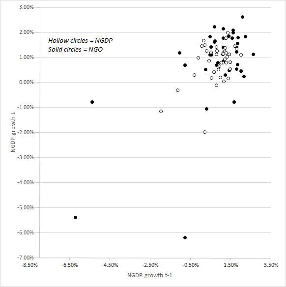
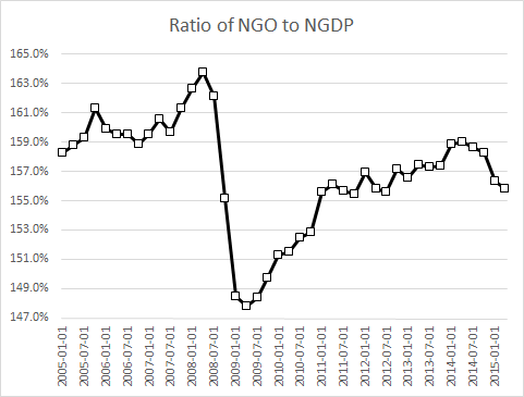
The recurring criticism in most posts is that NGO is volatile over the period when the data is available (2005Q1-today). True, the average growth rate of NGO is the same as NGDP over the same period, but the standard deviation is nearly twice that of NGDP. However if you exclude the initial shock of the recession, the standard deviations converge. In a way, all the difference in volatility between the two series is driven by the shock of the recession. Another way to see it is to recompute two graphs. One is an imitation of the graphs by Nunes where NGDP growth in period T is compared with growth in the period T minus 1, but we add NGO. The second is the ratio of NGO to NGDP.
As one can see from the first figure, NGO and NGDP show the same relation except for a cluster of points at the bottom for NGO. All of those lower points are related to the drop from the initial recession. All concentrated at the bottom. This suggests that the recession had a much deeper effect than otherwise believed. The second graph allows us to see it.
The ratio of NGO to NGDP shows that the two evolved roughly the same way over the period before the recession. However, when the recession hit, the drop was more important and the ratio never recovered! This suggest a much deeper deviation from the long-term trend of nominal spending which is not seen at the final level but would be seen rather in the undertaking of long-term projects and the formation of intangible capital (the areas that NGDP cannot easily capture).
The case for NGO over NGDP is solid. It does not alter the validity of the case for nominal spending stability. However since the case for nominal spending stability hinges on total transactions of inputs and outputs more than it does on the final goods sold, NGO is a better option.
Quick comment in response to Rognlie
In his reply to Nick Rowe, Matt Rognlie states that the more important fall of NGO is explained by changes in relative prices. Although his transformation shows this, the BEA disagrees. Here is the explanation provided by the BEA:
For example, value added for durable-goods manufacturing dropped 15 percent in 2009, while gross output dropped 19 percent. The decline in gross output is much more pronounced than the decline in value added because it includes each of the successive declines in the intermediate inputs supply chain required to manufacture the durable goods.
Was Murphy Foolish to Take Caplan’s Bet?
A few days ago, Bryan Caplan posted on his bet with Robert Murphy regarding inflation. Murphy predicted 10% inflation. He lost … big time. However, was he crazy to make that bet? In other words, what could explain Caplan’s victory?
Murphy was not alone in predicting this, I distinctly remember a podcast between Russ Roberts and Joshua Angrist on this where Roberts tells Angrist he expected high inflation back in 2008. Their claims were not indefensible. Central banks were engaging in quantitative easing and there was an important increase of the state money supply. There was a case to be made that inflation could surge.
It did not. Why?
In a tweet, Caplan tells me that monetary transmission channels are much more complex than they used to be and that the TIPS market knew this. Although I agree with both these points, it does not really explain why it did not materialize. I am going to propose two possibilities of which I am not fully convinced myself but whose possibility I cannot dismiss out of hand.
Imagine an AS-AD graph. If Murphy had been right, we should have seen aggregate demand stimulated to a point well above that of long-run equilibrium. Yet, its hard to see how quantitative easing did not somehow stimulate aggregate demand. Now, if aggregate demand was falling and that quantitative easing merely prevented it from falling, this is what would prove Murphy wrong. However, all of this assumes no movement of supply curves.
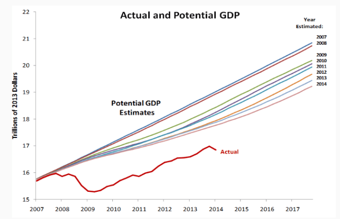
While AD falls and before monetary policy kicks in, imagine that policies are adopted that reduce the potential for growth and productivity improvement. In a way, this would be the argument brought forward by people like Casey Mulligan in work on labor supply and the “redistribution recession” and Edward Prescott and Ellen McGrattan who argue that, once you account for intangible capital, the real business cycle model is still in play (there was a TFP shock somehow). This case would mean that as AD fell, AS fell with it. I would find it hard to imagine that AS shifted left faster than AD. However, a relatively smaller fall of AS would lead to a strong recession without much deflation (which is what we have seen in this recession). Personally, I think there is some evidence for that. After all, we keep reducing the estimate for potential GDP everywhere while the policy uncertainty index proposed by Baker, Bloom and Davids shows a level change around 2008. Furthermore, there has been a wave – in my opinion of very harmful regulations – which would have created a maze of administrative costs to deal with (and whose burden is heavy according to Dawson and Seater in the Journal of Economic Growth). That could be one possibility that would explain why Murphy lost.
There is a second possibility worth considering (and one which I find more appealing): the role of financial regulations. Now, I may have been trained mostly by Real Business Cycle guys, but I do have a strong monetarist bent. I have always been convinced by the arguments of Steve Hanke and Tim Congdon (I especially link Congdon) and others that what you should care about is not M1 or M2, but “broad money”. As Hanke keeps pointing out, only a share of everything that we could qualify broadly as “money” is actually “state money”. The rest is “private money”. If a wave of financial regulations discourages banks to lend or incite them to keep greater reserves, this would be the equivalent of a drop of the money multiplier. If those regulations are enacted at the same time as monetary authorities are trying to offset a fall in aggregate demand, then the result depends on the relative impact of the regulations. The data for “broad money” (Hanke defines it as M4) shows convincingly that this is a potent contender. In that case, Murphy’s only error would have been to assume that the Federal Reserve’s policy took place with everything else being equal (which was not the case since everything seemed to be moving in confusing directions).

In the end, I think all of these explanations have value (a real shock, a banking regulation shock, an aggregate demand shock). In 25 years when economic historians such as myself will study the “Great Recession”, they will be forced to do like they do with Great Depression: tell a multifaceted story of intermingled causes and counter-effects for which no single statistical test can be designed. When cases like these emerge, it’s hard to tell what is happening and those who are willing to bet are daredevils.
P.S. I have seen the blog posts by Scott Sumner and Marcus Nunes regarding my NGO /NGDP claims. They make very valid points and I want to take decent time to address them, especially since I am using the blogging conversation as a tool to shape a working paper.
NGDP, NGO and total expenditures
I did not think that my post on NGO versus NGDP would gather attention, but it did (so, I am happy). Nick Rowe of Carleton University and the (always relevant) blog Worthwhile Canadian Initiative responded to my post with the following post (I was very happy to see a comment by Matt Rognlie in there).
Like Mr. Rowe, I prefer to speak about trade cycles as well. I do not know how the shift from “transactions” to “output” occurred, but I do know that as semantic as some may see it, it is crucial. While a transaction is about selling a unit of output, the way we measure output does not mean that we focus on all transactions. I became aware of this when reading Leland Yeager (just after reading about the adventures on Lucas’ Islands). However, Nick (if I may use first names) expresses this a thousand times better than I did in my initial post. When there is a shift of the demand for money, this will affect all transactions, not only those on final goods. Thus, my first point: gross domestic product is not necessarily the best for monetary transaction.
In fact, as an economist who decided to spend his life doing economic history, I do not like gross domestic product for measuring living standards as well (I’ll do a post on this when I get my ideas on secular stagnation better organized). Its just the “least terrible tool”. However, is it the “least terrible” for monetary policy guidance?
My answer is “no” and thus my proposition to shift to gross output or a measure of “total spending”. Now, for the purposes of discussion, let’s see what the “ideal” statistic for “total spending” would be. To illustrate this, let’s take the case of a change in the supply of money (I would prefer using a case with the demand for money, but for blogging purposes, its easier to go with supply)
Now unless there is a helicopter drop*, changes in the money supply generate changes in relative prices and thus the pattern (and level) of production changes too. Where this occurs depends on the entry point of the increased stock of money. The entry point could be in sectors producing intermediary goods or it could closer to the final point of sale. The closer it is to the point of sale, the better NGDP becomes as a measure of total spending. The further it is, the more NGDP wavers in its efficiency at any given time. This is because, in the long-run, NGDP should follow the same trend at any measure of total spending but it would not do so in the very short-run. If monetary policy (or sometimes regulatory changes affecting bank behavior “cough Dodd-Frank cough”) causes an increase in the production of intermediary goods, the movements the perfect measure of total spending would be temporarily divorced from the movements of NGDP. As a result, we need something that captures all transaction. And in a way, we do have such a statistic: input-output tables. Developed by the vastly underrated (and still misunderstood in my opinion) Wassily Leontief, input-output tables are the basis of any measurement of national income you will see out there. Basically, they are matrixes of all “trades” (inputs and outputs) between industries. What this means is that input-output tables are tables of all transactions. That would be the ideal measure of total spending. Sadly, these tables are not produced regularly (in Canada, I believe there are produced every five years). Their utility would be amazing: not only would we capture all spending (which is the goal of a NGDP target), but we could capture the transmission mechanism of monetary policy and see how certain monetary decisions could be affecting relative prices.** If input-output tables could be produced on a quarterly-basis, it would be the amazing (but mind-bogglingly complex for statistical agencies).
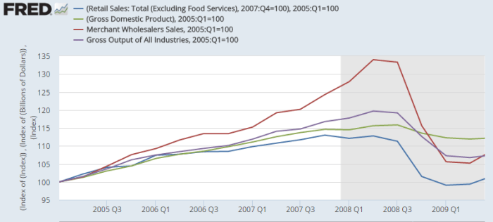
The closest thing, at present, to this ideal measure is gross output. It is the only quarterly statistic of gross output (one way to calculate total spending) that exists out there. The closest things are annual datasets. Yet, even gross output is incomplete as a measure of total spending. It does not include wholesale distributors (well, only a part of their activities through value-added). This post from the Cobden Centre in England details an example of this. Mark Skousen in the Journal of Private Enterprise published a piece detailing other statistics that could serve as proxies for “total spending”. One of those is Gross Domestic Expenditures and it is the closest thing to the ideal we would get. Basically, he adds wholesale and retail sales together. He also looks at business receipts from the IRS to see if it conforms (the intuition being that all sales should imitate receipts claimed by businesses). His measure of domestic expenditure is somewhat incomplete for my eyes and further research would be needed. But there is something to be said for Skousen’s point: total nominal spending did drop massively during the recession (see the fall of wholesale, gross output and retail) while NGDP barely moved while, before the recession, total nominal spending did increase much faster than NGDP.
In all cases, I think that it is fair to divide my claim into three parts: a) business cycles are about the deviation from trends in total volume of trades/transactions, thus the core variable of interest is nominal expenditures b) NGDP is not a measure of total nominal spending whose targeting the market monetarist crowd aims to follow; c) since we care about total nominal spending, what we should have is an IO table … every month and d) the imperfect statistics for total spending show that the case made that central banks fueled spending above trend and then failed to compensate in 2008-2009 seems plausible.
Overall, I think that the case for A, B and C are strong, but D is weak…
* I dislike the helicopter drop analogy. Money is never introduced in an equal fashion leading to a uniform price increase. It is always introduced through a certain number of entry points which distort relative prices and then the pattern of trade (which is why there is a positive short-term relation between real output and money supply). The helicopter drop analogy is only useful for explaining the nominal/real dichotomy for introductory macro classes.
** Funny observation here: if I am correct, this means that Hayek’s comments about the structure of production would have been answered by using Leontief’s input-output table. Indeed, the Austrians and Neoclassicals of the RBC school after them have long held that monetary policy’s real effects are seen through changes in the structure of production (in the Austrian jargon) or by inciting more long-term projects to be undertaken creating the “time to build” problem (in the RBC jargon). Regardless of which one you end up believing (I confess to a mixed bag of RBC/Austrian views with a slight penchant to walk towards Rochester), both can be answered by using input-output tables. The irony is that Hayek actually debated “planning” in the 1970s and castigated Leontief for his planning views. Although I am partial (totally) to Hayek’s view on planning, it is funny that the best tool (in my opinion) in support of Hayek is produced by an intellectual adversary
The Problem with Modern Monetary Theory
“Modern Monetary Theory,” a doctrine about fiat money, has captured the attention of some reformers and progressives. This doctrine – a set of propositions contrary to logic and evidence – purports to explain why the US and other economies are ailing, but is beset by contradictions with the historic facts and within the doctrine.
For example, The New Inquiry on 11 April 2014 featured an article by Rebecca Rojer on “The World According to Modern Monetary Theory.” The author regards it as a revelation of MMT that the “rules of money are not immutable laws of nature.” Since the science of economics explains the effects of incentives and decisions, evidently these money “rules” are the outcomes of private and governmental decisions, and since the effects are not immutable laws, people can arbitrarily create whatever outcomes they wish. That would indeed be wonderful, to just print money are thereby eliminate unemployment, depressions, and poverty, all without creating price inflation, because the rules of money creation are not immutable, so we can have whatever outcome we wish!
Science is based on logic and evidence rather than “revelations.” It is possible that there have been revelations, but these create religion rather than science, since if an experience or experiment cannot be duplicated, the revelations are not sufficient for scientific warrants. Various religions have had different revelations, and the members do not believe the revelations of the others.
The author provides an example of the MMT doctrine. Suppose there is an island that has minerals. The owner of the mines hires workers and pays them with fiat money, like the paper and bank-account money we have today, i.e. money created out of nothing. But the owner also imposes a tax on the wages of the miners. So evidently this mine owner is a government, and we are not dealing with private enterprise, but a coercive socialist state. The miners work enough to both pay the wage tax and be able to survive.
But a premise of this MMT island example is that prior to the mining, the people were able to hunt and farm without working too hard. So why would anyone work in the mines? The historical explanation is the “enclosures” movement, in which land that was held by small-scale farmers or by villages was forcibly taken by the aristocracy or by the state or by foreign invaders. This is not a money story, but a land-grab story. Another way to get forced labor, other than chattel slavery, is to require the payment of taxes in money, which forces subsistence farmers to work on plantations at least long enough to pay the taxes. That is more a tax story than a money story, since if the government insists on being paid in coconuts, and a farmer does not grow coconuts, he must work on the coconut plantation, get paid in coconuts, and then pay the tax. Therefore the forced labor is based on the government’s restrictions on alternative employment opportunities.
MMT is correct in stating that one way that the government gets people to accept its fiat money is what economists call the “fiscal theory of money,” that the government reinforces its money as a medium of exchange by requiring the use of that money for paying taxes. However, if the government currency is being hyper-inflated, taxpayers would keep their savings in, say, gold, or a stable foreign currency, and then convert it to the fiat money only when a tax payment is due. The fiscal effect only works if the government is not creating too much inflation.
Therefore MMT is incorrect as stating, as a “core building block,” that forcing people to pay taxes with fiat money “gives it its value.” That was not the case, for example, in Zimbabwe, which suffered hyperinflation. One “immutable” economic law of money is that the creation of money, beyond what is needed for transactions, results in price inflation, and the payment of taxes becomes tied to that inflation, via the nominal rise of prices and wages, rather than preventing inflation.
A related fallacy of MMT is that “sovereigns” in general create money by “spending it into existence.” That can indeed happen, as for example in the Zimbabwe hyperinflation, but in the US and most countries today, government spending comes from taxes and borrowing, not money creation. The central bank, such as the Federal Reserve, does not create money by spending it for goods, but rather by buying bonds and then increasing the banks’ reserves or funds to pay for the bonds.
Since the “core” proposition of MMT, that price inflation can be controlled by government’s taxing and spending, is incorrect, the whole superstructure of the MMT doctrine built on it collapses. Actually, MMT does accept the proposition that monetary inflation creates price inflation, but that true proposition contradicts the core MMT premise that tax-paying gives money its value.
A worse MMT fallacy is that the taxes paid to the government destroys money. MMT tells us that governments create money when they spend, and then the money disappears when taxes are paid. But a tax no more destroys money than the dollars used to buy bread. The seller of bread now has the money, and the government now has the dollars paid in taxes, and they then spend that money.
There have been various theories and doctrines on money and banking in the history of economic thought, and in my judgment, the explanations that best fit the facts are a combination of the monetarist and the Austrian schools of thought. The monetarist core is the equation MV=PT, which explains that the quantity of money (M) multiplied by its annual velocity or turnover (V) equals the price level (P) multiplied by the amount of transactions (T) measured in money. Thus high price inflation, a rise in P, is usually caused by monetary inflation, an on-going increase in M.
The Austrian school explains how excessive monetary inflation not only cause price inflation, but distorts relative prices, such as when house purchase prices rise faster than rentals. Austrian theory shows how governmental central planning fails because the knowledge to do so well is always lacking, and that applies to money as well. Hence the Austrians propose free-market money and banking, so that the market sets interest rates and the money supply.
Indeed the Fed failed to prevent the Great Depression of the 1930s and the Great Recession of 2008, and its policies generated high inflation during the 1970s and the cheap credit that has fueled land-value bubbles. MMT cannot do any better, because, as the Austrian theory explains, the optimal money supply is not only not known, but not knowable. The pure free market provides the optimal money supply just as it provides the optimal amount of bread and the optimal amount of shoes.
Around the Web: Nobel Prize Edition
I just got three of them.
- Why we need to separate the central bank from the monetary authority.
- “Market Design”
- Noble Matching.
Maybe one of our in-house economists can share their thoughts on the award this year as well…
