The great global trend for the equality of well-being since 1900

Some years ago, I read The Improving State of the World: Why We’re Living Longer, Healthier, More Comfortable Lives on a Cleaner Planet by Indur Goklany. It was my first exposition to the claim that, globally, there has been a long-trend in the equality of well-being. The observation made by Goklany which had a dramatic effect on me was that many countries who were, at the time of his writing, as rich (incomes per capita) as Britain in 1850 had life expectancy and infant mortality levels well superior to 1850 Britain. Ever since, I accumulated the statistics on that regard and I often tell my students that when comes the time to “dispell” myths regarding the improvement in living standards since circa 1800 (note: people are generally unable to properly grasp the actual improvement in living standards).

Some years after, I discovered the work of Leandro Prados de la Escosura who is a cliometrician who (I think I told him that when I met him) influenced me deeply in my work regarding the measurement of living standards and who wrote this paper which I will discuss here.  His paper, and his work in general, shows that globally the inequality in incomes has faltered since the 1970s.  That is largely the result of the economic rise of India and China (the world’s two largest antipoverty programs). Figure1Leandro

However, when extending his measurements to include life expectancy and schooling in order to capture “human development” (the idea that development is not only about incomes but the ability to exercise agency – i.e. the acquisition of positive liberty), the collapse in “human development” inequality (i.e. well-being) precedes by many decades the reduction in global income inequality. Indeed, the collapse started around 1900, not 1970!

Figure2LEandro.png

In reading Leandro’s paper, I remembered the work of Goklany which had sowed the seeds of this idea in my idea. Nearly a decade after reading Goklany’s work well after I fully accepted this fact as valid, I remain stunned by its implications. You should too.

Nightcap

  1. The new age of great power politics John Bew, New Statesman
  2. Before We Cure Others of Their False Beliefs, We Must First Cure Our Own Christopher Preble, Cato Unbound
  3. Libertarians (FDP) ruin coalition talks in Germany Christian Hacke, Deutsche Welle
  4. The Rich You Will Always Have With You Brandon Turner, Law & Liberty

On the “tea saucer” of income inequality since 1917

I disagree often with the many details that underlie the arguments of Thomas Piketty and Emmanuel Saez. That being said, I am also a great fan of their work and of them in general. In fact, I think that both have made contributions to economics that I am envious to equal. To be fair, their U-curve of inequality is pretty much a well-confirmed fact by now: everyone agrees that the period from 1890-1929 was a high-point of inequality which leveled off until the 1970s and then picked up again.

Nevertheless, while I am convinced of the curvilinear aspect of the evolution of income inequality in the United State as depicted by Piketty and Saez, I am not convinced by the amplitudes. In their 2003 article, the U-curve of inequality really looks like a “U” (see image below).  Since that article, many scholars have investigated the extent of the increase in inequality post-1980 (circa). Many have attenuated the increase, but they still find an increase (see here here here here here here here here here). The problem is that everyone has been considering the increase – i.e. the right side of the U-curve. Little attention has been devoted to the left side of the U-curve even though that is where data problems should be considered more carefully for the generation of a stylized fact. This is the contribution I have been coordinating and working on for the last few months alongside John Moore, Phil Magness and Phil Schlosser. 

Blog Figure

To arrive at their proposed series of inequality, Piketty and Saez used the IRS Statistics of Income (SOI) to derive top income fractiles. However, the IRS SOI have many problems. The first is that between 1917 and 1943, there are many years where there are less than 10% of the potential tax population that files a tax return. This prohibits the use of a top 10% income share in many years unless an adjustment is made. The second is that prior to 1943, the IRS reports net income and reports adjusted gross income after 1943. As such, to link post-1943 with pre-1943, there needs to be an additional adjustment. Piketty and Saez made some seemingly reasonable assumptions, but they have never been put to the test regarding sensitivity and robustness. This is leaving aside issues of data quality (I am not convinced IRS data is very good as most of it was self-reported pre-1943 which is a period with wildly varying tax rates). The question here is “how good” are the assumptions?

What we did is verify each assumption to see their validity. The first one we tackle is the adjustment for the low number of returns. To make their adjustments, Piketty and Saez used the fact that single households and married households filed in different quantities relative to their total population. Their idea is that a year in which there was a large number of return was used, the ratio of single to married could be used to adjust the series. The year they used is 1942. This is problematic as 1942 is a war year with self-reporting when large quantities of young American males are abroad fighting. Using 1941, the last US peace year, instead shows dramatically different ratios. Using these ratios knocks off a few points from the top 10% income share. Why did they use 1942? Their argument was there was simply not enough data to make the correction in 1941.  They point to a special tabulation in the 1941 IRS-SOI of 112,472 1040A forms from six states which was not deemed sufficient to make to make the corrections. However, later in the same document, there is a larger and sufficient sample of 516,000 returns from all 64 IRS collection districts (roughly 5% of all forms). By comparison, the 1942 sample Piketty and Saez used to correct only had 455,000 returns.  Given the war year and the sample size, we believe that 1941 is a better year to make the adjustment.

Second, we also questioned the smoothing method to link net income-based series with adjusted-gross income based series (i.e. pre-1943 and post-1943 series). The reason for this is that the implied adjustment for deductions made by Piketty and Saez is actually larger than all the deductions claimed that were eligible under the definition of Adjusted Gross Income – which is a sign of overshot on their parts. Using the limited data available for deductions by income groups and making some assumptions (very conservative ones) to move further back in time, we found that adjusting for “actual deductions” yields a lower level of inequality. This is contrasted with the fixed multipliers which Piketty and Saez used pre-1943.

Third, we question their justification for not using the Kuznets income denominator. They argued that Kuznets’ series yielded an implausible figure because, in 1948, its use yielded a greater income for non-fillers than for fillers.  However, this is not true of all years. In fact, it is only true after 1943. Before 1943, the income of non-fillers is equal in proportion to the one they use post-1944 to impute the income of non-fillers. This is largely the result of an accounting error definition. Incomes before 1943 were reported as net income and as gross incomes after that point. This is important because the stylized fact of a pronounced U-curve is heavily sensitive to the assumption made regarding the denominator.

These three adjustments are pretty important in terms of overall results (see image below).  The pale blue line is that of Piketty of Saez as depicted in their 2003 paper in the Quarterly Journal of Economics. The other blue line just below it is the effect of deductions only (the adjustment for missing returns affects only the top 10% income share). All the other lines that mirror these two just below (with the exception of the darkest blue line which is the original Kuznets inequality estimates) compound our corrections with three potential corrections for the denominators. The U-curve still exists, but it is not as pronounced. When you look with the adjustments made by Mechling et al. (2017) and Auten and Splinter (2017) for the post-1960 period (green and red lines) and link them with ours, you can still see the curvilinear shape but it looks more like a “tea saucer” than a pronounced U-curve.

In a way, I see this as a simultaneous complement to the work of Richard Sutch and to the work of Piketty and Saez: the U-curve still exists, but the timing and pattern is slightly more representative of history. This was a long paper to write (and it is a dry read given the amount of methodological discussions), but it was worth it in order to improve upon the state of our knowledge.

FigureInequality

On Monopsony and Legal Surroundings

A few days ago, in reply to this December NBER study, David Henderson at EconLog questioned the idea that labor market monopsonies matter to explain sluggish wage growth and rising wage inequality. Like David, I am skeptical of this argument. However, I am skeptical for different reasons.

First, let’s point out that the reasoning behind this story is well established (see notably the work of Alan Manning). Firms with market power over a more or less homogeneous labor force which must assume a disproportionate amount of search costs have every incentive to depress wages. This can lead to reductions in growth as, notably, it discourages human capital formation (see these two papers here and here as examples). As such, I am not as skeptical of “monopsony” as an argument.

However, I am skeptical of “monopsony” as an argument. Well, what I mean is that I am skeptical of considering monopsony without any qualifications regarding institutions. The key condition to an effective monopsony is the existence of barriers (natural and/or legal to mobility). As soon as it is relatively easy to leave a small city for another city, then even a city with a single-employer will have little ability to exert his “market power” (Note: I really hate that word). If you think about it simply through these lenses, then all that matters is the ability to move. All you need to care about are the barriers (legal and/or natural) to mobility (i.e. the chance to defect).

And here’s the thing. I don’t think that natural barriers are a big deal. For example, Price Fishback found that the “company towns” im the 19th century were hardly monopsonies (see here, here, here and here). If natural barriers were not a big deal, they are certainly not a big deal today. As such, I think the action is largely legal. My favorite example is the set of laws adopted following the Emancipation of slaves in the United States which limited the mobility (by limiting the chances of Northerners hiring agents to come who would act as headhunters in the South). That is a legal barrier (see here and here). I am also making that argument regarding the institution of seigneurial tenure in Canada in a working paper that I am reorganizing (see here).

What about today? The best example are housing restrictions? Well, housing construction and zoning regulations basically make the supply of housing quite inelastic. The areas where these regulations are the most severe are also, incidentally, high productivity areas. This has two effects on mobility. The first is that low-productivity workers in low-productivity areas cannot easily afford to move to the high-productivity area. As such, you are reducing their options of defection and increasing the likelihood that they will not look. You are also reducing the pool of places to apply which means that, in order to find a more remunerative job, they must search longer and harder (i.e. you are increasing their search costs). The second effect is that you are also tying workers to the areas they are in. True, they gain because the productivity becomes capitalized in the potential rent from selling any property they own. However, they are in essence tied to the place. As such, they can be more easily mistreated by employers.

These are only examples. I am sure I could extend the list to reach the size of the fiscal code (well, maybe not that much). The point is that “monopsony” (to the extent that it exists) is merely a symptom of other policies that either increase search costs for workers or reduce the number of options for defections. And I do not care much for analyzing symptoms.

In the Search for an Optimal Level of Inequality

Recently, the blog ThinkMarkets published a post by Gunther Schnabl about how Friedrich Hayek’s works helped to understand the link between Quantitative Easing and political unrest. The piece of writing summarized with praiseworthy precision three different stages of Friedrich Hayek’s economic and political ideas and, among the many topics it addressed, it was mentioned the increasing level of income and wealth inequality that a policy of low rates of interest might bring about.

It is well-known that Friedrich Hayek owes the Swedish School as much as he does the Austrian School on his ideas about money and capital. In fact, he borrows the distinction between natural and market interest rates from Knut Wicksell. The early writings of F.A. Hayek state that disequilibrium and crisis are caused by a market interest rate that is below the natural interest rate. There is no necessity of a Central Bank to arrive at such a situation: the credit creation of the banking system or a sudden change of the expectancies of the public could set the market interest rate well below the natural interest rate and, thus, lead to what Hayek and Nicholas Kaldor called “the Concertina Effect.”

At this point we must formulate a disclaimer: Friedrich Hayek’s theory of money and capital was so controversial and subject to so many regrets by his early supporters – like said Kaldor, Ronald Coase, or Lionel Robbins – that we can hardly carry on without reaching a previous theoretical settlement over the apportations of his works. Until then, the readings on Hayek’s economics will have mostly a heuristic and inspirational value. They will be an starting point from where to spring new insights, but hardly a single conclusive statement. Hayekian economics is a whole realm to be conquered, but precisely, the most of this quest still remains undone.

For example, if we assume – as it does the said post – that ultra-loose monetary policy enlarges inequality and engenders political instability, then we are bound to find a monetary policy that delivers, or at least does not avoid, an optimal level of inequality. As it is explained in the linked lecture, the definition of such a concept might differ whether it depends on an economic or a political or a moral perspective.

Here is where I think the works of F.A. Hayek have still so much to give to our inquiries: the matter is not where to place an optimal level of inequality, but to discover the conditions under which a certain level of inequality appears to us as legitimate, or at least tolerable. This is not a subject about quantities, but about qualities. Our mission is to discover the mechanism by which the notions of fairness, justice, or even order are formed in our beliefs.

Perhaps that is the deep meaning of the order or equilibrium that it is reach when, to use the terminology of Wicksell and Hayek’s early writings, both natural and market interest rates are the same: a state of affairs in which the most of the expectancies of the agents could prove correct. The solution does not depend upon a particular public policy, but on providing an abstract institutional structure in which each individual decision could profit the most from the spontaneous order of human interaction.

Is the U-curve of US income inequality that pronounced?

For some time now, I have been skeptical of the narrative that has emerged regarding income inequality in the West in general and in the US in particular. That narrative, which I label UCN for U-Curve Narrative, simply asserts that inequality fell from a high level in the 1910s down to a trough in the 1970s and then back up to levels comparable to those in the 1910s.

To be sure, I do believe that inequality fell and rose over the 20th century.  Very few people will disagree with this contention. Like many others I question how “big” is the increase since the 1970s (the low point of the U-Curve). However, unlike many others, I also question how big the fall actually was. Basically, I do think that there is a sound case for saying that inequality rose modestly since the 1970s for reasons that are a mixed bag of good and bad (see here and here), but I also think that the case that inequality did not fall as much as believed up to the 1970s is a strong one.

The reasons for this position of mine relates to my passion for cliometrics. The quantitative illustration of the past is a crucial task. However, data is only as good as the questions it seek to answer. If I wonder whether or not feudal institutions (like seigneurial tenure in Canada) hindered economic development and I only look at farm incomes, then I might be capturing a good part of the story but since farm income is not total income, I am missing a part of it. Had I asked whether or not feudal institutions hindered farm productivity, then the data would have been more relevant.

Same thing for income inequality I argue in this new working paper (with Phil Magness, John Moore and Phil Schlosser) which is a basically a list of criticisms of the the Piketty-Saez income inequality series.

For the United States, income inequality measures pre-1960s generally rely on tax-reporting data. From the get-go, one has to recognize that this sort of system (since it is taxes) does not promote “honest” reporting. What is less well known is that tax compliance enforcement was very lax pre-1943 and highly sensitive to the wide variations in tax rates and personal exemption during the period. Basically, the chances that you will report honestly your income at a top marginal rate of 79% is lower than had that rate been at 25%. Since the rates did vary from the high-70s at the end of the Great War to the mid-20s in the 1920s and back up during the Depression, that implies a lot of volatility in the quality of reporting. As such, the evolution measured by tax data will capture tax-rate-induced variations in reported income (especially in the pre-withholding era when there existed numerous large loopholes and tax-sheltered income vehicles).  The shift from high to low taxes in the 1910s and 1920s would have implied a larger than actual change in inequality while the the shift from low to high taxes in the 1930s would have implied the reverse. Correcting for the artificial changes caused by tax rate changes would, by definition, flatten the evolution of inequality – which is what we find in our paper.

However, we go farther than that. Using the state of Wisconsin which had a tax system with more stringent compliance rules for the state income tax while also having lower and much more stable tax rates, we find different levels and trends of income inequality than with the IRS data (a point which me and Phil Magness expanded on here). This alone should fuel skepticism.

Nonetheless, this is not the sum of our criticisms. We also find that the denominator frequently used to arrive at the share of income going to top earners is too low and that the justification used for that denominator is the result of a mathematical error (see pages 10-12 in our paper).

Finally, we point out that there is a large accounting problem. Before 1943, the IRS provided the Statistics of Income based on net income. After 1943, there shift between definitions of adjusted gross income. As such, the two series are not comparable and need to be adjusted to be linked. Piketty and Saez, when they calculated their own adjustment methods, made seemingly reasonable assumptions (mostly that the rich took the lion’s share of deductions). However, when we searched and found evidence of how deductions were distributed, they did not match the assumptions of Piketty and Saez. The actual evidence regarding deductions suggest that lower income brackets had large deductions and this diminishes the adjustment needed to harmonize the two series.

Taken together, our corrections yield systematically lower and flatter estimates of inequality which do not contradict the idea that inequality fell during the first half of the 20th century (see image below). However, our corrections suggest that the UCN is incorrect and that there might be more of small bowl (I call it the Paella-bowl curve of inequality, but my co-authors prefer the J-curve idea).

InequalityPikettySaez.png

Can we trust US interwar inequality figures?

This question is the one that me and Phil Magness have been asking for some time and we have now assembled our thoughts and measures in the first of a series of papers. In this paper, we take issue with the quality of the measurements that will be extracted from tax records during the interwar years (1918 to 1941).

More precisely, we point out that tax rates at the federal level fluctuated wildly and were at relatively high levels. Since most of our inequality measures are drawn from the federal tax data contained in the Statistics of Income, this is problematic. Indeed, high tax rates might deter honest reporting while rapidly changing rates will affect reporting behavior (causing artificial variations in the measure of market income). As such, both the level and the trend of inequality might be off.  That is our concern in very simple words.

To assess whether or not we are worrying for nothing, we went around to find different sources to assess the robustness of the inequality estimates based on the federal tax data. We found what we were looking for in Wisconsin whose tax rates were much lower (never above 7%) and less variable than those at the federal levels. As such, we found the perfect dataset to see if there are measurement problems in the data itself (through a varying selection bias).

From the Wisconsin data, we find that there are good reasons to be skeptical of the existing inequality measured based on federal tax data. The comparison of the IRS data for Wisconsin with the data from the state income tax shows a different pattern of evolution and a different level (especially when deductions are accounted for). First of all, the level is always inferior with the WTC data (Wisconsin Tax Commission). Secondly, the trend differs for the 1930s.

Table1 for Blog

I am not sure what it means in terms of the true level of inequality for the period. However, it suggests that we ought to be careful towards the estimations advanced if two data sources of a similar nature (tax data) with arguably minor conceptual differences (low and stable tax rates) tell dramatically different stories.  Maybe its time to try to further improve the pre-1945 series on inequality.

From the Comments: Weber, Geloso on inequality

How did I not see these before? Rick chimed in on Zak’s post about inequality and libertarianism awhile back. As usual, he tries to give the opposition the benefit of the doubt:

Taking public choice logic seriously means considering the political distortions/impediments to proposed policy. Taking inequality seriously is the flip side of that. Perceptions of (and attitudes towards) inequality matter and libertarians (and conservatives) would do well to acknowledge it.

I suspect that the problem is that 1) (like any ideology) we’ve got a blind spot, and inequality is in that spot. 2) Our liberal friends can see into that blind spot. 3) They’ve got a blind spot that leads them to make silly policy prescriptions (e.g. ignoring public choice roots of inequality and instead calling for policies that would reduce growth). And as a result, 4) we’re turned off by discussion of inequality before considering it.

Vincent, in the usual French manner, has a different take:

Okay massive disagreement here:

A: Inequality is not something “measurable” in the sense of utility. I chose to be an economist. My income is X% below that of my wife who went to school fewer years than I did and her income grows faster than mine and she will live longer than me (in probabilistic terms given life expectancy differences M/F). According to that definition, my couple is an unequal one and growing more unequal. Yet, I would not trade her job for mine even if her job was twice as remunerative (she is an attorney). I chose a path of lesser income because it made me happy. Income maximization was, in that case, not synonymous with utility maximization. By definition, rich societies will have more cases like that since gains in marginal utility may not be associated with marginal gains in monetary income. See the issue of the backward-bending labor supply curve.

B: The literature on linking growth to inequality is VERY weak. Look at the empirical papers, the results often depend on the choice of variables and the time window. It NEVER accounts for what I mentioned in point A. More importantly, there is NO THEORETICAL LINK with neoclassical theory on this (with the notable exception of Herb Gintis and Sam Bowles and I am working on a paper tackling their logic) that is axiomatically consistent. An empirical observation without a theory that is logically sound (the most repeated is the general Keynesian argument about consumption, but that is very weak and that rebuttal is powerful in the theoretical papers) is basically rubbish.

C: The Great Gatsby Curve is also rubbish since most of the past observations are based on the weird assumptions that mobility based on father-sons is a proper estimate to compare with modern estimates. You can consult the very convincing rebuttals made by Scott Winship. Moreover, the Great Gatsby curve is again a case of empirical observations without theory. I don’t need any of this story to see that mobility is down (modestly) at the same time that labor market restrictions are up.

There is more discussion, too.

Did Inequality Fall During the Great Depression ?

Inequality

The graph above is taken from Piketty and Saez in their seminal 2003 article in the Quarterly Journal of Economics. It shows that inequality fell during the Great Depression. This is a contention that I have always been very skeptical of for many reasons and which has been – since 2012 – the reason why I view the IRS-data derived measure of inequality through a very skeptical lens (disclaimer: I think that it gives us an idea of inequality but I am not sure how accurate it is).

Here is why.

During the Great Depression, unemployment was never below 15% (see Romer here for a comparison prior to 1930 and this image derived from Timothy Hatton’s work). In some years, it was close to 25%. When such a large share of the population is earning near zero in terms of income, it is hard to imagine that inequality did not increase. Secondly, real wages were up during the Depression. Workers who still had a job were not worse off, they were better off. This means that you had a large share of the population who saw income reductions close to 100% and the remaining share saw actual increases in real wages. This would push up inequality no questions asked. This could be offset by a fall in the incomes from profits of the top income shares, but you would need a pretty big drop (which is what Piketty and Saez argue for).

There is some research that have tried to focus only on the Great Depression. The first was one rarely cited NBER paper by Horst Mendershausen from 1946 who found modest increases in inequality from 1929 to 1933. The data was largely centered on urban data, but this flaw works in favor of my skepticism as farm incomes (i.e. rural incomes) fell more during the depression than average incomes. There is also evidence, more recent, regarding other countries during the Great Depression. For example, Hungary saw an increase in inequality during the era from 1928 to 1941 with most of the increase in the early 1930s. A similar development was observed in Canada as well (slight increase based on the Veall dataset).

Had Piketty and Saez showed an increase in inequality during the Depression, I would have been more willing to accept their series with fewer questions and doubts. However, they do not discuss these points in great details and as such, we should be skeptical.

A hidden cost of the war on drugs

AI just completed another paper (this time with my longtime partner in crime Vadim Kufenko) where we question an hypothesis advanced by Samuel Bowles regarding the cost of inequality. In the process, we proposed an alternative explanation which has implications for the evaluation of the war on drugs.

In recent years, Samuel Bowles (2012) has advanced a theory (well-embedded within neoclassical theoretical elements while remaining elegantly simple) whereby inequality increases distrust which in turn magnifies agency problems. This forces firms to expend more resources on supervision and protection which means an expansion of the “guard labor force” (or supervisory labor force). Basically, he argues there is an over-provision of security and supervision. That is the cost of inequality which Bowles presents as a coordination failure. We propose an alternative explanation for the size of the guard and supervisory labor forces.

Our alternative is that there can be over-provision of security and supervision, but this could also be the result of a government failure. We argue that the war on drugs leads to institutional decay and lower levels of trust which, in turn, force private actors to deploy resources to supervise workers and protect themselves. Basically, efforts at prohibiting illicit substances require that limited policing resources be spread more thinly which may force private actors to expend more resources on security for themselves (thus creating an overprovision of security). This represents a form of state failure, especially if the attempts at policing these illicit substances increase the level of crime to which populations are vulnerable. To counteract this, private actors invest more in protection and supervision.

Using some of the work of Jeffrey Miron and Katherine Waldock, we show that increases in the intensity of prohibition enforcement efforts (measured in dollars per capita) have significant effects on the demand for guard labor. Given that guards represent roughly 1 million individuals in the US labor market, that is not a negligible outcome. We find that a one standard deviation increase in the level of drug enforcement efforts increases the ratio of guards to the population by somewhere between 12.92% and 13.91% (which is the equivalent of roughly 100,000 workers).

While our paper concentrated on proposing an alternative to the argument advanced by Bowles regarding the cost of inequality, we (more or less accidentally) measured a hidden cost from the war on drugs. The insecurity (increased crime rates and spillovers from illegal markets into formal markets) brought forth by drug prohibition  forces an over-provision of security and supervision (our supervision measure which includes workers that supervise other workers were smaller than with the security guard measure).

Basically, a hidden (private cost) of the war on drugs is that we must reallocate resources that we could have used otherwise. Its a little like when I say that it is meaningless to compare healthcare expenditures to GDP in Canada and the United States because Canadians assume costs in a hidden manner through rationing. Waiting lists in Canada are longer than in the US. The cost is lost wages and enduring pain and that cost will not appear in measures of expenditures to GDP. The war on drugs works the same way. There is a fiscal cost (expenditures dedicated to it and the taxes that we must impose), there is a crime cost (destruction of lives and property) and there is a reallocation cost of privately providing security which is hard to measure.

*The paper is available here. 

Did 89% of American Millionaires Disappear During the Great Depression?

Over the years, I became increasingly skeptical of using tax data to measure inequality. I do not believe that there is no value in computing inequality with those sources (especially after the 1960s, the quality is much better in the case of the US). I simply believe that there is a great need for prudence in not overstretching the results. This is not the first time I make this point (see my paper with Phil Schlosser and John Moore here) and I think it is especially crucial for anything prior to 1943 (the introduction of tax withholding).

One of my main point is that the work of Gene Smiley which ended up published in the Journal of Economic History has generally been ignored. Smiley had highlighted many failings in the way the tax data was computed for measuring inequality. His most important point was that tax avoidance foiled the measurements of top incomes and how well they could transposed on the overall national accounts.

More precisely, Smiley argued that the tax shelters of the 1920s and 1930s would have affected reporting behavior. As long as corporations could issue stock dividends rather than cash dividends, delaying the payment of dividends until shareholders were in lower tax brackets, there would be avoidance. Furthermore, state and municipal securities were exempted from taxation which meant that taxpayers could shelter income and end up in lower brackets. All this combined to wide fluctuations in marginal tax rates conspires to reduce the quality of the tax data in computing inequality. Rather than substantial increases in inequality, Smiley found that his corrected estimates (which kept tax rates constant) suggested no increase in inequality during the 1920s and a minimal decrease when you exclude capital gains.

Alongside John Moore, Phil Schlosser and Phil Magness, I am in the process of attempting to extend the Smiley corrections to include everything up to 1941 (Smiley had ended in 1929). As a result, I had to assemble the tax data and the tax rates and I was surprised to see that, even without regressions, we can see the problem of relying on the tax data for the interwar period.

The number of millionaires in the tax reports is displayed below. As one can see, it is very low from 1917 to 1924 – a period of high tax rates. However, as tax rates fell in the 1920s, the number of millionaires quintupled. And then, when the Depression started in synchronicity with the increases in top marginal tax rates, it went back down. It went down by 89% from 1929 to 1941. Now, I am quite willing to entertain that many millionaires were wiped out during the Great Depression. I am not willing to entertain the idea that 9 out of every 10 millionaires disappeared. What I am willing to entertain is that the tax data is clearly and heavily problematic for the pre-withholding era.* This is evidence in favor of caution and prudence in interpreting inequality measures derived from tax data.


taxreports

I am of those who believe that inequality was lower than reported elsewhere in the 1920s, higher than reported in the 1930s and 1940s. Combined together, these would mean that inequality would tend to follow a L-curve or a J-curve from the 1920s up to the present rather than the U-curve often reported.  I will post more on this as my paper with Moore, Schlosser and Magness progresses. 

On Gentrification, Inequality and Zoning

On the CityLab blog, Richard Florida posted a piece pointing out that gentrification has virtually no effects on homeowners. I can buy that result, especially since I wrote a policy piece for a think tank back in the summer of 2016 on the issue. The important point that Florida underlines (by citing a paper by Martin and Beck in Urban Affairs Review) is that homeowners are not being displaced, but renters are more likely to be. This will probably fuel some people who are concerned about inequality. I disagree.

I want to point out that my interest in the issue is entirely related to the issue of inequality which some individuals have tried to tie to gentrification (sometimes without understanding that causality can run both ways). If you want to tie the two issues together, then you must realize that there are four “types” of gentrification. First of all, gentrification always appear in an area that is poor and it is always a result of a shift in demand for land in that area. However, that area can be largely unoccupied or heavily inhabited. It can also be in a district where zoning is lax or burdensome. In each of these situations, you will different effects with different interpretations for inequality.

  • Scenario 1 (largely vacant, lax zoning laws): in this situation, demand shifts right but there is slack in the local housing market and in any case, supply can adjust easily. In that case, the effects on rents will be minimal and will probably be smaller than the economic gains in terms of local economic activity. In this situation, there is little displacement and there is in fact a reduction in inequality.
  • Scenario 2 (largely vacant, heavy zoning laws): same happens, except that the restrictions on construction and building conversions put a ceiling on the capacity of a local area to adapt. The effect on rents is ambiguous and depends largely on the relative quantity changes (how many people relative to empty units). There are probably small to moderate gains in the area. There are ambiguous effects on inequality.
  • Scenario 3 (heavily occupied, lax zoning laws): in this situation, the influx of individuals creates a temporary surge in rents. This is because, in the short-term, housing supply is inelastic. In the long-run, the supply is more elastic and new units can be added to counterbalance the price effects. So, there is a long-term benefit that comes after a small bump. More individuals will be displaced than in scenario 1. Overall, a reduction in inequality might occur.
  • Scenario 4 (heavily occupied, heavy zoning laws): in this situation, the influx happens in a market where the supply is highly inelastic (short and long-run). In that case, the shift in demand creates a substantial increase in rents. This is where gentrification can hurt and be tied to inequality.

These four scenarios are important because they show something important that some people have to understand. Gentrification can increase inequality. However, that depends on the context and the institutions (zoning) surrounding the area in which it happens. In all cases, gentrification is a normal process that can’t really be stopped but turns sour because of zoning laws. Thus, if you really want to tie gentrification to inequality, it should twice removed since the first parents are zoning laws and construction limits.

What is Wrong with Income Inequality? Five Reasons to be Concerned

I sometimes part ways with many of my libertarian and classical liberal friends in that I do have some amount of tentative concern for income/wealth inequality (for the purposes of this article, the otherwise important economic distinction between the two is not particularly relevant since the two are strongly correlated with each other). Many libertarians argue that inequality ultimately doesn’t matter. There is good reason to think this drawing from the classic arguments of Nozick and Hayek about how free exchange in a market economy can often interrupt preferred distributions.

The argument goes like this: take whatever your preferred distribution of income is, be it purely egalitarian or some sort of Rawlsian distribution such that the distribution benefits only the worst off in society. Assume there is one individual in the economy who has some product or service everyone wants to buy (in Nozick’s example it was Wilt Chamberlain playing basketball), and let everyone pay a relatively small amount of income to that one individual. For example, assume you have a society with 10,000 people all who start off with an equal endowment of $5 and all of them decide to pay Wilt Chamberlain $1 to watch him play basketball. Very few people would object to those individual exchanges, yet at the end Wilt Chamberlain ends up with $10,005 dollars and everyone else has $4, and our preferred distribution of income has been grossly upset even though the individual actions that led to that distribution are not objectionable. In other words, allowing for free exchange precludes trying to construct an optimal result of that free exchange (a basic consequence of recognizing spontaneous order).

Further, these libertarians argue, it is more important to ensure that the poor are better off in absolute terms than to ensure they are better off relative to their wealthier peers. Therefore, if a given policy will increase the wealth of the wealthiest by 10% and the poorest by 5%, there is no reason to oppose this policy on the grounds that it increases inequality because the poor are still made richer. Therefore, it is claimed, we should focus on policies that improve economic growth and the incomes of the poor and be indifferent as to its impact on relative inequality, since those policies are strongly correlated with bettering the economic conditions of the poor. In fact, as Mises Argued in Liberalism and the Classical Tradition, a certain amount of inequality is necessary for markets to function: they create a market for luxury goods that can be experimented and developed into future mass-consumption goods everyone can consume. Not everyone could afford, for an example, an IPod when it first came out, however today MP3 players are cheap and plentiful because the very wealthy were able to demand it when it was very expensive.

I agree with my libertarians in thinking that this argument is largely correct, however I do not think it proves, as Hayek argued, that social justice (understood in this context as distributive justice) is a “mirage” or that we should be altogether unconcerned with wealth or income distributions. All this argument does is mean that there is no overall deontological theory for an ideal income distribution, but there still might be good consequentialist reasons to think that excessively unequal distributions can impact many of the things that classical liberals tell us to worry about, such as the earnings of the poor, more free political economic outcomes, or overall economic growth. Further, even on Nozick’s entitlement theory of justice, we might oppose income inequality if it arises through unjust means. Here are five reasons why libertarians and classical liberals should be concerned about income inequality (note that they are mostly empirical reasons, not claims about the nature of justice):

1) Income Inequality as a Result of Rent Seeking

Certain government policies result in uneven income distribution. For an example, a paper by Patrick MacLaughlin and Lauren Stanley at the Mercatus Center empirically analyze the regressive effects of regulatory policy. Specifically, Stanley and MacLaughlin find that high barriers to entry create barriers to entry which worsens income mobility. Poorer would-be entrepreneurs cannot enter the market if they must, for an example, pay thousands of dollars for a license, or spend a large amount of time getting costly education and certifications to please some regulatory bureaucracy. This was admitted even by the Obama Administration in a recent report advising reform of occupational licensing laws. As basic public choice theory teaches, regulators are subject to regulatory capture, in which established business interests lobby regulators to erect barriers to entry to harm would-be competitors. Insofar as inequality is a result of such rent-seeking, libertarians have an obvious reason to oppose it.

Many other policies can worsen inequality. When wealthy corporations receive artificial monopolies from policies such as excessive intellectual property laws, insulating them from competition or when they gain wealth at the expense of poorer taxpayers through improper subsidies. When the government uses violent policing tactics to unequally enforce drug laws against poorer communities, or when it uses civil asset forfeiture to take the property of the worst off. When the government uses eminent domain to take the property of disadvantaged individuals and communities in the name of public works projects, or when they implement minimum wage laws that displace low-skilled workers. Or, if the structure of welfare benefits discourages income mobility, which also worsens inequality. There are a myriad of bad government policies which benefit the rich and exploit the poor, some of which are a direct result of rent-seeking on behalf of the wealthy.

If the rich are getting richer, or if the poor are stopped from becoming wealthier, as a result of government coercion, even Nozick’s entitlement theory of justice calls for us to be skeptical of the resulting income distribution. As Matt Zwolinski argues, income distributions are not only a result of, pace Nozick, a result of the free exchanges of individuals, but they are also a result of the institutions in which those individuals exchange. Insofar as inequality is a result of unjust institutions, we have good reason to call that inequality unjust.

Of course, that principle is still very hard to empirically apply. It is hard to tell how much of an unequal distribution is a function of bad institutions and how much is a function of free exchange. However, this means we can provide very limited theories of distributive justice not as constructivist attempts to mold market outcomes to our moral desires, but as rough rules of thumb. If it is true that unequal distributions are a function of bad institutions, then unequal distributions should cause us to re-evaluate those institutions.

2) Income Inequality and Government Exploitation
Of course, many with more Marxist inclinations will argue that any amount of economic inequality will inherently result in class-based exploitation. There are very good, stand-by classical liberal (and neoclassical economic) reasons to reject this as Marxian class analysis as it depends on a highly flawed labor theory of value. However, that does not mean there is not some correlation between some notion of macro-level exploitation of the worst-off and high levels of inequality which libertarians have good reason to be concerned about, for reasons closely related to rent-seeking. Those with a high amount of economic power, particularly in western democracies, are very likely to also have a strong influence over the policies set by the government. There is reason to fear that this will create a class of wealthy people who, through political rent-seeking channels discuss earlier, will control state policies and institutions to protect their interests and wealth at the expense of the worst-off in society. Using state coercion to protect oneself at the expense of others is, under any understanding of the term, coercion. In this way, income inequality can beget rent-seeking and regressive policies which lead to more income inequality which leads to more rent-seeking, leading to a vicious political-economic cycle of exploitation and increasing inequality. In fact, even early radical classical liberal economists applied theories of class analysis to this type of problem.

3) Inequality’s Impacts on Economic Growth

There is a robust amount of empirical literature suggesting that excessive income inequality can harm economic growth. How? The Economist explains:

Inequality could impair growth if those with low incomes suffer poor health and low productivity as a result, or if, as evidence suggests, the poor struggle to finance investments in education. Inequality could also threaten public confidence in growth-boosting policies like free trade, says Dani Rodrik of the Institute for Advanced Study in Princeton.

Of course, this is of special concern to consequentialist classical liberals who claim we should worry mostly about the betterment of the poor in absolute terms, since economic growth is strongly correlated with bettering living standards. There is even some reason for these classical liberals, given their stated normative reasons, to (at least in the short-term given that we have unjust institutions) support some limited redistributive policies, but only those that are implemented well and don’t worsen inequality or growth (such as a Negative Income Tax), insofar as it boosts growth and helps limited the growth of rent-seeking culture described with reasons one and two.

4) Inequality and Political Stability

There is further some evidence that income inequality increases political instability. If the poor perceive that current distributions are unjust (however wrong they may or may not be), they might have social discontent. In moderate scenarios, (as the Alsenia paper I linked to argue) this can lead to reduced investment, which aggravates third problem discussed earlier. In some scenarios, this can lead to support for populist demagogues (such as Trump or Bernie Sanders) who will implement bad policies that not only might harm the poor but also limit individual liberty in other important ways. In the most extreme scenarios (however unlikely, but still plausible), it can lead to all-out violent revolutions and warfare. At any rate, libertarians and classical liberals concerned with ensuring tranquility and freedom should be concerned if inequality increases.

5) Inequality and Social Mobility

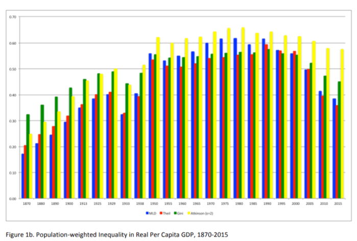
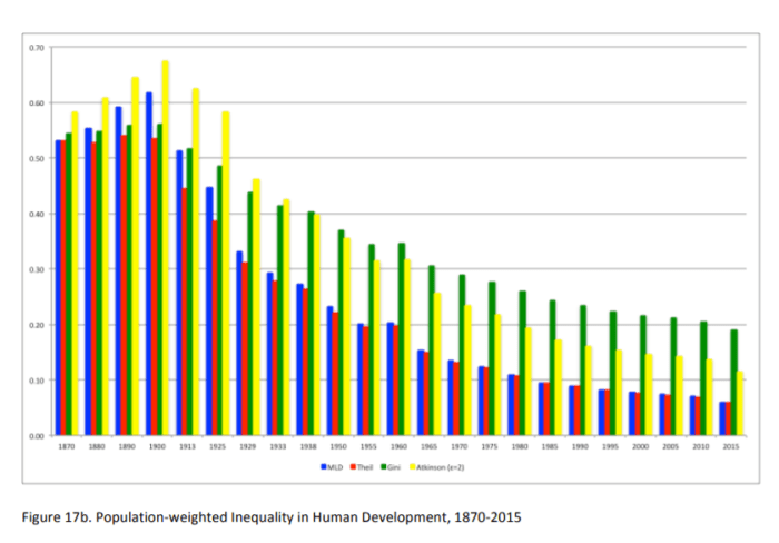
More meritocratic-leaning libertarians might say we should be concerned about equal opportunities rather than equal outcomes. There is some evidence that the two are greatly linked. In particular, the so-called “Great Gatsby Curve,” which shows a negative relationship between economic mobility and income inequality. In other words, unequal outcomes can undermine unequal opportunities. This can be because higher inequality means unequal access to certain services, eg. Education, that can enable social mobility, or that the poorer may have fewer connections to better-paying opportunities because of their socio-economic status. Of course, there is likely some reverse causality here; institutions that limit social mobility (such as those discussed in problem one and two) can be said to worsen income mobility intergenerationally, leading to higher inequality in the future. Though teasing out the direction of causality empirically can be challenging, there is reason for concern here if one is concerned about social mobility.

The main point I’m getting at is nothing new: one need not be a radical leftist social egalitarian who thinks equal economic outcomes are necessarily the only moral outcomes to be concerned on some level with inequality. How one responds to inequality is empirically dependent on the causes of the problems, and we have some good reasons to think that more limited government is a good solution to unequal outcomes.

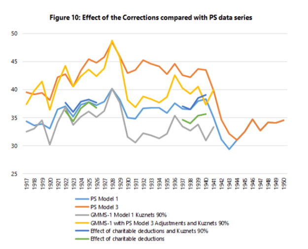
This is not to say inequality poses no problem for libertarians’ ideal political order: if it is the case that markets inherently beget problematic levels of inequality, as for example Thomas Piketty claims, then we might need to re-evaluate how we integrate markets. However, there is good reason to be skeptical of such claims (Thomas Piketty’s in particular are suspect). Even if we grant that markets by themselves do lead to levels of inequality that cause problems 3-5, we must not commit the Nirvana fallacy. We need to compare government’s aptitude at managing income distribution, which for well-worn public choice reasons outlined in problems one and two as well as a mammoth epistemic problem inherent in figuring out how much inequality is likely to lead to those problems, and compare it to the extent to which markets do generate those problems. It is possible (very likely, even) that even if markets are not perfect in the sense of ensuring distribution that does not have problematic political economic outcomes, the state attempting to correct these outcomes would only make things worse.

But that is a complex empirical research project which obviously can’t be solved in this short blog post, suffice it to say now that though libertarians are right to be skeptical of overarching moralistic outrage about rising levels of inequality, there are other very good empirical reasons to be concerned.

Canadian Megatrends: Top 1% income share and median age

Statistics Canada just came up with a study on the top income share of the top 1% in Canada. As I have explained elsewhere, my view of inequality is that: a) it has increased; b) not as much as we think; c) a lot of the increase is from desirable factors (personal utility maximization differing from income maximization or international immigration) or neutral factors (demography, marriage); d) that the inequality that is worrisome stems either from birth or government manipulations of the market and; e) that those stemming from government manipulations, direct (like subsidizing firms) or indirect (like the war on drugs which means that a large number of individuals are jailed and then released with a “prison earnings penalty” which stymies their income levels and growth), are the easiest to fight.

The recent Statistics Canada study allows me to make my point again with regards to element C of my answer. As I looked at their series, all I could think was “median age”. A lot of the variations seem to be related to the median age of the population. I went back to the census data I had collected for my book and plotted it against the data. This is what it looks like.

medianage

Why would there be a relation? Well, each year you measure the income distribution, the demographic structure of that population changes. As it grows older, you have more people at the top of their earnings curve relative to those at the bottom. Not only that, but earnings curve seem elongated in recent times – we live longer and so some people work older as witnessed by increased labor force participation rates above a certain age closer to retirement. And the heights of the earnings curve are now higher than ever before while we also enter later into the labor market.

Now, I am not sure how much aging would “explain away” rising inequality in Canada, but there is no point denying that it does explain some of it away. But, I would not be surprised that a large part is explained away. Why am I saying that? Because of this paper on Norway’s age structure. 

In Norway, the median age in 1950 was much higher than it was in Canada back then and today, it is roughly the same as Canada (although Canada has had a steeper increase in inequality). And according to the paper on Norway, adjusting for composition bias in inequality measures caused by aging, eliminates entirely the upward trend in that country. In fact, it may even reverse the trend whereby inequality adjusted for age has actually declined over time. This is a powerful observation. Given that Canada has had a steeper increase in median age, this suggests that the increase in inequality might be simply the cause of a statistical artifice.

The most depressing thing with Chetty et al.

The Chetty et al. paper has been on my mind over the weekend (see Saturday’s post). The one thing that has moved more or less in line with the absolute mobility measure of Chetty et al. has been…the size of government.

I know that as soon as some of you read the last four words on the previous paragraphs, your eyes rolled. However, even from a social-democratic perspective, it is depressing! It is not the first time I make this observation.   In the pages of Essays in Economic and Business HistoryI recently reviewed Unequal Gains (authored by Peter Lindert and Jeffrey Williamson and published at Princeton University Press) and I observed that the “great leveling” they observed from the 1910s to the 1970s had a lot to do with the northward migration of American blacks, the closing of the gender wage gap and the convergence of the southern states. I also observed that the increase in inequality in the United States after 1970 occurred at the same time as an the state grew more in size and scope (see blog post here).

However, as I mentioned elsewhere, I am very skeptical of the tax-based data on inequality in the United States and I am afraid to push that point. However, the Chetty et al. data provides further confirmation: trends in inequality/social mobility deteriorates as the state becomes more active (see the graph below).

sizegov

Now, I am aware that the causality can cut both ways. It may be that inequality (economic mobility) is rising (falling) in spite of increasing state action, it may be that state action is fueling the the rise (reduction) of inequality (economic mobility) or it may be that the state has no effects whatsoever on the evolution. Regardless of which of the three viewpoints you tend to adopt (I lean towards a mixture the second option – see my paper with Steve Horwitz here which is under consideration for publication), the implications are immensely depressing with regards to social policy in the last 75 years.