A flaw regarding the chance of “out-earning” your parents

When Raj Chetty publishes a paper, it generally comes with a splash. The last one is no exception. His paper (co-authored), picked up by David Leonhardt at the New York Times and Justin Wolfers on Twitter, basically measures the American dream : what are your chances to do better than your parents. The stunning conclusion is that someone born in 1940 had a 90%+ chance of “out-earning” his parents compared with a few points above 50% for those born in the 1980s. I am not convinced. Well, when I am not convinced, I am saying I am not convincing about how big the drop is! I think the drop is smoother (the slope of decline is gentler) and the starting point for the 1940 cohort is too high.  As a big fan of Chetty, I must press this point.

More precisely, I am saying that the bar (income threshold) over which someone had to jump in 1940 is underestimated and overestimated in 1980. Setting the bar too low (high) means very high (low) chances of “out-earning” your parents. To set the bar too low, you must underestimate (overestimate) the income of the parents.  This could occur if household economies of scale are not accounted for.

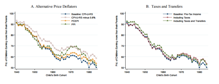
An income of 30,000$ for 3 persons is not the same as an income of 60,000$ for 6 peoples. On a per capita basis, the income is the same. But, if you adjust for economies of scale in housing and furnitures, there are differences (the simplest is square root).  This gives you income per adult equivalent. Chetty et al. are aware of that and they provided a sensitivity analysis which is not mentioned by those who are relaying the article. Since household size has tended to fall over time, the growth in per capita income is faster than the growth in income per adult equivalent (a better measure). Any correction for this long-term demographic trend would attenuate the slope of the decline of the chance to out-earn your parents. And indeed, once Chetty et al. make the correction, the decline is much more modest (but still present – see below).

size

Simultaneously, Chetty et al. also present other important sensitivity checks. All of them relevant. But, in a strange decision, Chetty et al. decided to isolate each of the sensitivity checks rather than compile them. Taken individual, they all seem minor – except adjusting for family size. But compound this with the other sensitivity check proposed by Chetty et al.: price deflators. Using the well-known bias in the the CPI that overestimates inflation by 0.8%, Chetty et al. find that, by the end of their perod, there is roughly a ten percentage point difference between the baseline uncorrected CPI and the corrected CPI (see below). Compound this with the corrections for family and you still get a decline – but again the slope of the decline is much more modest. If you add panel B from figure 3 in Chetty et al – which includes taxes and transfers – you probably get a few extra points up. There will still probably be a decline, but a moderate one.

pricetaxes

Finally, at footnote 19, Chetty et al. also point out that they do not account for in-kind transfers prior to 1967 (there were some).  And, on page 13, they point out that “one may be concerned that levels of absolute mobility for recent cohorts may still be understated because of increases in fringe benefits, nonmarket goods, or under-reporting of income in the CPS”. Add in all these little extra problems to the family size, the transfers and the inflation correction and I am not sure how big the drop from 1940 to the end of the studied period is. Finally, I would also add that an understudied point in economic history is what the distribution of in-kind payments according to income was. From studying the British industrial revolution, I have generally to see that it is the poorest workers who receive in-kind payments (which are not measured) and the richest receive much fewer of those in proportion of their incomes. One of the few to note that distributional was the hardcore left-leaning scholar Gabriel Kolko who mentioned this issue in Dissent back in the 1950s.  If Kolko is correct, then the income of “poor parents” in 1940 is underestimated. As a result, the bar over which the children of said parents must jump is set mildly too low. If that is the case, the odds for the 1940 birth cohort are overestimated.

Combine all of these things together and I am not sure that the drop is as dramatic as many are making it out to be. I would be very satisfied if Chetty et al. would publish all the corrections they did and do a sensitivity check with hypothetical regarding a sliding-scale of in-kind payments in 1940 according to income (10% of income for poorest to 0% for the richest). I would just like to see how much it matters.

Testing the High-Wage Economy (HWE) Hypothesis

Over the last week or so, I have been heavily involved in a twitterminar (yes, I am coining that portemanteau term to designate academic discussions on twitter – proof that some good can come out of social media) between myself, Judy Stephenson , Ben Schneider , Benjamin Guilbert, Mark Koyama, Pseudoerasmus,  Anton Howes (whose main flaw is that he is from King’s College London while I am from the LSE – nothing rational here), Alan Fernihough and  Lyman Stone. The topic? How suitable is the “high-wage economy” (HWE) explanation of the British industrial revolution (BIR).

Twitter debates are hard to follow and there is a need for summaries given the format of twitter. As a result, I am attempting such a summary here which is laced with my own comments regarding my skepticism and possible resolution venues.

An honest account of HWE

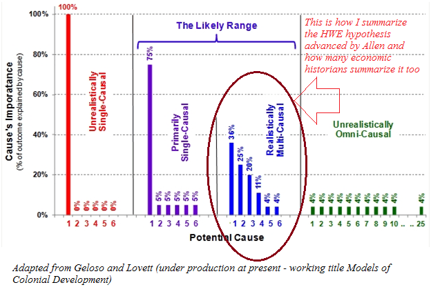
First of all, it is necessary to offer a proper enunciation of HWE’s role in explaining the industrial revolution as advanced by its main proponent, Robert Allen.  This is a necessary step because there is a literature attempting to use high-wages as an efficiency wage argument. A good example is Morris Altman’s Economic Growth and the High-Wage Economy  (see here too) Altman summarizes his “key message” as the idea that “improving the material well-being of workers, even prior to immediate increases in productivity can be expected to have positive effects on productivity through its impact on economic efficiency and technological change”. He also made the same argument with my native home province of Quebec relative to Ontario during the late 19th century. This is basically a multiple equilibria story. And its not exactly what Allen advances. Allen’s argument is that wages were high in England relative to energy. This factors price ratio stimulated the development of technologies and industries that spearheaded the BIR. This is basically a context-specific argument and not a “conventional” efficiency wage approach as that of Allen. There are similarities, but they are also considerable differences. Secondly, the HWE hypothesis is basically a meta-argument about the Industrial Revolution. It would be unfair to caricature it as an “overarching” explanation. Rather, the version of HWE advanced by Robert Allen (see his book here) is one where there are many factors at play but there is one – HWE – which had the strongest effects. Moreover, while it does not explain all, it was dependent on other factors that contributed independently.  The most common view is that this is mixed with Joel Mokyr’s supply of inventions story (which is what Nick Crafts has done). In the graph below, the “realistically multi-causal” explanation is how I see HWE. In Allen’s explanation, it holds the place that cause #1 does. According to other economists, HWE holds spot #2 or spot #3 and Mokyr’s explanations holds spot #1.

hwe

In pure theoretical terms (as an axiomatic statement), the Allen model is defensible. It is a logically consistent construct. It has some questionnable assumptions, but it has no self-contradictions. Basically, any criticism of HWE must question the validity of the theory based on empirical evidence (see my argument with Graham Brownlow here) regarding the necessary conditions. This is the hallmark of Allen’s work: logical consistency. His work cannot be simply brushed aside – it is well argued and there is supportive evidence. The logical construction of his argument requires a deep discussion and any criticism that will convince must encompass many factors.

Why not France? Or How to Test HWE

As a doubter of Allen’s theory (I am willing to be convinced, hence my categorization as doubter), the best way to phrase my criticism is to ask the mirror of his question. Rather than asking “Why was the Industrial Revolution British”, I ask “Why Wasn’t it French”. This is what Allen does in his work when he asks explicitly “Why not France?” (p.203 of his book). The answer proposed is that English wages were high enough to justify the adoption of labor-saving technologies. In France, they were not. This led to differing rates of technological adoptions, an example of which is the spinning jenny.

This argument hinges on some key conditions :

  1. Wages were higher in England than in France
  2. Unit labor costs were higher in England than in France (productivity-adjusted wages) (a point made by Kelly, Mokyr and Ó Gráda)
  3. Market size factors are not sufficiently important to overshadow the effects of lower wages in France (R&D costs over market size mean a low fixed cost relative to potential market size)
  4. The work year is equal in France as in England
  5. The cost of energy in France relative to labor is higher than in England
  6. Output remained constant while hours fell – a contention at odds with the Industrious Revolution which the same as saying that marginal productivity moves inversely with working hours

If most of these empirical statements hold, then the argument of Allen holds. I am pretty convinced by the evidence advanced by Allen (and E.A. Wrigley also) regarding the low relative of energy in England. Thus, I am pretty convinced that condition #5 holds. Moreover, given the increases in transport productivity within England (here and here), the limited barriers to internal trade (here), I would not be surprised that it was relatively easy to supply energy on the British market prior to 1800 (at least relative to France).

Condition #3 is harder to assess in terms of important. Market size, in a Smithian world, is not only about population (see scale effects literature). Market size is a function of transaction costs between individuals, a large share of which are determined by institutional arrangements. France has a much larger population than England so there could have been scale effects, but France also had more barriers to internal trade that could have limited market size. I will return to this below.

Condition #1,2,4 are basically empirical statements. They are also the main points of tactical assault on Allen’s theory.  I think condition #1 is the easiest to tackle. I am currently writing a piece derived from my dissertation showing that – at least with regards to Strasbourg – wages in France presented in Allen (his 2001 article) are heavily underestimated (by somewhere between 12% and 40% using winter workers in agriculture and as much as 70% using the average for laborers in agriculture). The work of Judy Stephenson, Jane Humphries and Jacob Weisdorf has also thrown the level and trend of British wages into doubts. Bringing French wages upwards and British wages downwards could damage the Allen story. However, this would not be a sufficient theory. Industrialization was generally concentrated geographically. If labor markets in one country are not sufficiently integrated and the industrializing area (lets say the “textile” area of Lancashire or the French Manchester of Mulhouse or the Caën region in Normandy) has uniquely different wages, then Allen’s theory can hold since what matters is the local wage rate relative to energy. Pseudoerasmus has made this point but I can’t find any mention of that very plausible defense in Allen’s work.

Condition #2 is the weakest point and given Robert Fogel’s work on net nutrition in France and England, I have no problem in assuming that French workers were less productive. However, the best evidence would be to extract piece rates in textile-producing regions of France and England. This would eliminate any issue with wages and measuring national productivity differences. Piece rates would perfectly capture productivity and thus the argument could be measured in a very straightforward manner.

Condition #4 is harder to assess and more research would be needed. However, it is the most crucial piece of evidence required to settle the issue once and for all. Pre-industrial labor markets are not exactly like those of modern days. Search costs were high which works in a manner described (with reservations) by Alan Manning in his work on monopsony but with much more frictions. In such a market, workers may be willing to trade in lower wage rates for longer work years. In fact, its like a job security argument. Would you prefer 313 days of work guaranteed at 1 shilling per day or a 10% chance of working 313 days for 1.5 shillings a day (I’ve skewed the hypothetical numbers to make my point)? Now, if there are differences in the structure of labor markets in France and England during the 18th and 19th centuries, there might be differences in the extent of that trade-off in both countries. Different average discount on wages would affect production methods. If French workers were prone to sacrifice more on wages for steady employment, it may render one production method more profitable than in England. Assessing the extent of the discount of annual to daily wages on both markets would identify this issue.

The remaining condition (condition #6) is, in my opinion, dead on arrival. Allen’s model, in the case of the spinning jenny, assumed that labor hours moved in an opposite direction as marginal productivity. This is in direct opposition to the well-established industrious revolution. This point has been made convincingly by Gragnolati, Moschella and Pugliese in the Journal of Economic History. 

In terms of research strategy, getting piece rates, proper wage estimates and proper labor supplied estimates for England and France would resolve most of the issue. Condition #3 could then be assessed as a plausibility residual.  Once we know about working hours, actual productivity and real wages differences, we can test how big the difference in market size has to be to deter adoption in France. If the difference seems implausible (given the empirical limitations of measuring effective market size in the 18th century in both markets), then we can assess the presence of this condition.

My counter-argument : social networks and diffusion

For the sake of argument, let’s imagine that all of the evidence favors the skeptics, then what? It is all well and good to tear down the edifice but we are left with a gaping hole and everything starts again. It would be great to propose a new edifice as the old one is being questioned. This is where I am very much enclined towards the rarely discussed work of Leonard Dudley (Mothers of Innovation). Simply put, Dudley’s argument is that social networks allowed the diffusion of technologies within England that fostered economic growth. He has an analogy from physics which gets the point across nicely. Matter has three states : solid, gas, liquid. Solids are stable but resist to change. Gas, matter are much more random and change frequently by interacting with other gas, but any relation is ephemeral. Liquids permit change through interaction, but they are stable enough to allow interactions to persist for some time. Technological innovation is like a liquid. It can “mix” things together in a somewhat stable form.

This is where one of my argument takes life. In a small article for Economic Affairs, I argued (expanding on Dudley) that social networks allowed this mixing (I am also expanding that argument in a working paper with Adam Martin of Texas Tech University). However, I added a twist to that argument which I imported from the work of Israel Kirzner (one of the most cited books in economics, but not by cliometricians – more than 7000 citations on google scholar). Economic growth, in Kirzner’s mind,  is the result of entrepreneurs discovering errors and arbitrage possibilities. In a way, growth is a process of discovering correcting errors. An analogy to make this point is that entrepreneurs look for profits where the light is while also trying to move the light to see where it is dark. What Kirzner dubs as “alertness” is in fact nothing else than repeated and frequent interactions. The more your interact with others, the easier it becomes for ideas to have sex. Thus, what matters is how easy it is for social networks to appear and generate cheap information and interactions for members without the problem of free riders. This is where the work of Anton Howes becomes very valuable. Howes, in his PhD thesis supervised by Adam Martin who is my co-author on the aforementioned project (summary here), showed that most innovators went in frequent with one another and they inspired themselves from each other. This is alertness ignited!

If properly harnessed, the combination of the works of Howes and Dudley (and also James Dowey who was a PhD student at the LSE with me and whose work is *Trump voice* Amazing) can stand as a substitute to Allen’s HWE if invalidated.

Conclusion

If I came across as bashing on Allen in this post, then you have misread me. I admire Allen for the clarity of his reasoning and his expositions (given that I am working on a funded project to recalculate tax-based measures in the US used by Piketty to account for tax avoidance, I can appreciate the clarity in which Allen expresses himself). I also admire him for wanting to “Go big or go home” (which you can see in all his other work, especially on enclosures). My point is that I am willing to be convinced of HWE, but I find that the evidence leans towards rejecting it. But that is very limited and flawed evidence and asserting this clearly is hard (as some of the flaws can go his way). Nitpicking Allen’s HWE is a necessary step for clearly determining the cause of BIR. It is not sufficient as a logically consistent substitute must be presented to the research community. In any case, there is my long summary of the twitteminar (officially trademarked now!)

P.S. Inspired by Peter Bent’s INET research webinar on institutional responses to financial crises, I am trying to organize a similar (low-cost) venue for presenting research papers on HWE assessment. More news on this later.

The Uniqueness of Italian Internal Divergence

A few weeks ago, I got engaged in a twitter debate with Garett Jones, Pseudoerasmus and Anna Missiaia (see her great work here) about institutions in Italy. During the course of that discussion, I was made aware that I held a false belief. Namely, the belief that since the late 19th century, there had only been a minor divergence within Italy. In reality, there has been considerable divergence within the country since the late 19th century.

In the wake of the Italian referendum, it is worth examining how big is this divergence. Below is a map of regional GDP per capita taken from Europa.ec.  The southern regions of Italy have GDP per capita below 75% of the European average while some of the northern regions have GDP per capita above 125% of the European average. The IStat database suggest similar levels of divergence across regions in Italy.

Gross_domestic_product_(GDP)_per_inhabitant_in_purchasing_power_standard_(PPS)_in_relation_to_the_EU-28_average,_by_NUTS_2_regions,_2014_(¹)_(%_of_the_EU-28_average,_EU-28_=_100)_RYB2016.png

So, how much divergence was there – say a little a more than one hundred years ago? Well, according to the great work of Felice (see here in the Economic History Review and here), there were more similarities back in the 19th century than there are today. Take the Liguria which – in 1891 – had per capita value added of 44% above national average. Take also Campania which was 3% below the national average. Today, the IStat data places Liguria 9% above national average but the region of Campania is 37% below the national average. Overall, regardless of how you present the data , divergence has increase. Just expressed at coefficient of variations, there has been an increase. In 1891, the coefficient of variation stood at 22.95% while it stood at 28.95% in 2013.

italiangdp

This makes Italy into an oddity. My own work shows that in Canada, since the 19th century, there has been considerable convergence (see article in Economics Bulletin). The same happened in the United States (see this paper by Michener and McLean), in England (here and here) and in Sweden (here). Among western countries, increased internal divergence is rare and Italy is the prime case example. And this is a strong indictment. Either Italy as a whole shares the same steady-state status and something is preventing upwards convergence from the South or Italy has two different economies with two different steady-states. In both cases, the implications are depressing.

England circa 1700: low-wage or high-wage

A few months ago, I discussed the work of my friend (and fellow LSE graduate) Judy Stephenson on the “high-wage economy” of England during the 18th century. The high-wage argument basically states that high wages relative to capital incite management to find new techniques of production and that, as a result, the industrial revolution could be initiated. Its a crude summary (I am not doing it justice here), but its roughly accurate.

In her work, Judy basically indicated that the “high-wage economy” observed in the data was a statistical artifact. The wage rates historians have been using are not wage rates, they’re contract rates that include an overhead for contractors who hired the works. The wage rates were below the contract rates in an amplitude sufficient to damage the high-wage narrative.

A few days ago, Jane Humphries (who has been a great inspiration for Judy and whose work I have been discretely following for years) and Jacob Weisdorf came out with a new working paper on the issue that have reinforced my skepticism of the wages regarding England. A crude summary of Humphries and Weisdorf’s paper goes as such: preindustrial labor markets had search costs, workers were willing to sacrifice on the daily wage rate (lower w) in order to obtain steady employment (greater L) and thus the proper variable of interest is the wage paid on annual contracts.

While their results do not affect England’s relative position (it only affects the trend of living standards in England), it shows that there are flaws in the data. These flaws should give us pause before proposing a strong theory like the “high-wage economy” argument. Taken together, the work of Stephenson (whom I am told is officially forthcoming), Humphries and Weisdorf show the importance of doing data work as the new data may overturn some key pieces of research (maybe, I am not sure, there is some stuff worth testing).

On granting the Nobel to Kirzner

In a little over a week, the Nobel Prize in economics will be unveiled. A part of me wishes that Robert Barro wins or maybe Dale Jorgenson or even William Baumol. However, I would be thrilled if Israel Kirzner won. Back in 2014, he was mentioned for the prize and it was the year that Jean Tirole, deservedly, won the prize. Since then, I have been dreaming of it as it would cement into the mainstream the best that the Austrian school of economics can offer.

Unlike many of colleagues, I have always had sympathies for numerous points made by the Austrians. Throughout my training, the Austrian school of economics was largely derided as cranks. Initially, I jumped on the bandwagon and I believed the Austrians to be crazy. However, I became exposed to many of their key points and like Edmund Phelps, I felt that the “best of the Austrians” could not be rejected so easily. True, there is some wheat to sort from the chaff, but the same applies for every school of thought.  I realized that most of their inputs in macroeconomics were largely incorporated in models like Lucas’ Islands Model or in Prescott’s Time to Build. However, what most intrigued me was how they used general equilibrium as a teaching tool, but not as a research tool. General equilibrium is useful for understanding key axiomatic assertions, but when you have an “applied economics” question, it is a hard tool to use – especially for an economic historian like me.

Kirzner is the perfect representation of the best that the Austrian school has to offer. In a way, his entire work can be summarized as such: it is the process leading to (new) equilibrium(s) that is the most interesting aspect of economics.

It is when I understood that insight that I finally grasped the deeper meaning of Hayek’s claim that “competition is a discovery process”. Entrepreneurs are people who look for the $100 bill on the sidewalk by innovating, by exploiting arbitrage opportunities and by discovering what consumers really want. They are constantly heading towards an equilibrium point. But as they try to do so, they shift the ability to produce and consume to greater levels and, in doing so, they generate a new equilibrium. And the process continues as long as human beings are humans.

For someone who studies economic history like I do, this is the most fruitful way of looking at social interactions. After all, the industrial revolution is everything except an equilibrium and the industrial revolution is most momentous structural break in history. The search for equilibrium and the creation of new equilibriums are by far more useful tools for questions like the end of “Malthusian pressures” or the beginning of the Industrial Revolution.

Of course, I am veering into excessive simplification of Kirzner’s contribution. But consider his book, Competition and Entrepreneurship. Alone, it has 7,362 citations (according to google scholar).  This is half the citations obtained by the most cited article in the American Economic Review (Armen Alchian and Harold Demsetz’s Production, Information Costs and Economic Organization). It’s close to 3,000 more citations that Deaton and Muellbauer’s “Almost Ideal Demand System” (4,775 citations). And Deaton won the Nobel last year!

By virtue of being affiliated with the Austrians, mainstream economists could have relegated him to obscurity. However, for such a citation count to be achieved, he must have been to showcase the best that the Austrian school has to offer. Just for that, maybe his contribution should be recognized.

Minorities and Economic Growth: Evidence from Jewish Communities in Premodern Europe

Urban theorist Richard Florida is celebrated for arguing that cities today succeed by attracting members of the “creative class.”  In a similar spirit I have a recent paper with Noel D. Johnson where we investigated whether or not cities in medieval and early modern Europe grew faster if they possessed a Jewish community.

Scholars have long noted the role of minority groups in economic development. This is particularly true for the the premodern period. The great scholar of long-run historical development in Europe, Fernand Braudel, observed that “successful merchants who controlled trade circuits and networks often belonged to foreign minorities.” These minorities could be other nationalities or religious minorities, for example, “the Jews, the Armenians, the Banyans, the Parsees, the Raskolniki (Old Believers) in Russia or the Christian Copts in Muslim Egypt” (Braudel, 1979, 1982, 165).

Hornung (2014) studies the impact of the Huguenot migration to Prussia. Since the nineteenth century, scholars like Friedrich List linked the presence of Huguenots with the transmission of human capital, skills, and innovation. Hornung (2014) is able to test this hypothesis using Prussian immigration lists from 1700 that document the location of Huguenot settlements and firm-level data on input and output for all 750 textile manufactories in Prussia in the year 1802. Approximately 16,000 to 20,000 Huguenots fled France to Prussia at the end of the seventeenth century.  Hornung finds that the presence of Huguenots significantly increased firm productivity. Specifically, a 1 percentage point increase in the share of Huguenots was associated with 1.5 percentage points higher productivity in 1802.

Jewish Communities and City Growth

In our paper we take a broad sweep of European history from 1400 to 1850.  We have a total of 1,792 cities in our panel data from the Bairoch (1988) dataset and 1,069 Jewish communities that appear in the Encyclopedia Judaica. The figure below shows both the cities in the Bairoch dataset and the Jewish communities mentioned in the Encyclopedia Judaica.


bairochandjewishcitiesgreyscale

To understand the relationship between the presence of a Jewish community and subsequent city growth we conduct a difference-in-differences style regression analysis.

The fact that we have data on city populations every century means we can hold constant the identity of a city using city fixed effects and see whether or not it grew faster in the centuries when it had a Jewish community in comparison to those centuries when it did not. We can also control for the possibility that overall city growth was faster in some centuries in comparison to others using century fixed effects.

We are also able to hold constant other factors that could plausibly have affected city growth. We control for local geography including cereal suitability, proximity to rivers, and proximity to coast, as these factors likely affected city growth in different ways over time. We also control for local infrastructure including presence of university and distance to a medieval trade route.

Our  analysis suggests that, indeed, cities with Jewish communities grew faster on average between 1400 and 1850. The effect we find suggests that cities with Jewish communities grew about one third faster than those that did not have Jewish communities. This analysis remains a correlation, however. We do not know if the presence of a Jewish community brought with it economic benefits or if Jews merely choose to settle in faster growing cities.

Instrumenting the Presence of a Jewish Community

We model the network of Jewish communities as one way to see whether the effect of Jews on city growth was indeed casual. By examining how Jewish communities expanded we hope to isolate a source of exogenous variation in the presence of a Jewish community.

We assume that a Jewish community is more likely to be established close to another Jewish community because of trade networks, financial relationships, or cultural linkages. We then calculate the closest travel path between Jewish communities using our information about the location of roads and river networks and estimates of premodern transport costs. The important assumption we make is that if cities with Jewish communities share certain “unobservable” characteristics that might make them more likely to grow rapidly, these characteristics become less correlated with distance.

We then divide Europe into 5km x 5km grids and assign the lowest travel cost to each grid. We apply Djikstra’s algorithm to determine the lowest cost of travel between all 3,211,264 city pairs (van Etten, 2012). This allows us to create a measure of ‘Jewish network access’ for each city.

Jewish network access itself is, of course, correlated with the unobservable characteristics of the city for which it is calculated. To overcome this we adopt two strategies to create valid instruments out of the network access measures. First, we calculate Jewish network access for cities that are only more than a certain distance away from each other. Second, we use information on expulsions to weight our measure of Jewish network access. The intuition behind this is that Jewish expulsions consist of an exogenous “push” factor leading to Jews settling in new cities close to the existing network of Jewish communities. Using these two strategies we obtain similar (though larger in magnitude) effects from the presence of a Jewish community on city growth. This provides further suggestive evidence that the correlation we found in our baseline analysis was indeed causal.

The Relationship Between Urban Growth and the Presence of a Jewish Community Over time

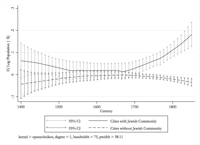
Across specifications, we find that cities with Jewish communities experienced no growth advantage in the 15th and 16th centuries. After 1600, however, they began to grow significantly faster.

motivationlpoly

The relationship we observe in the Figure does not appear to be inline with a pure human capital story. Jews had higher human capital than Christians throughout the medieval and early modern period. But the growth advantage of cities that had Jewish communities only became evident after 1600. This raises the possibility that something else changed around  17th century that made the human capital and skills of Jews more complementary to economic growth.

Two Mechanisms: Jewish Emancipation and Market Access

The two factors that stand out in explaining the emergence of a growth advantage for cities with Jewish communities after 1600 but not before are: (1) Jewish Emancipation after 1750; and (2) a complementarity between the presence of a Jewish community and market access.

The process of Jewish emancipation began in continental Europe after 1780. It was a major institutional break that signified a major change in the economic, social, and political status of the Jews in Europe. In work with Jean-Paul Carvalho, I’ve shown that Jewish emancipation lead to a religious schism and the emergence of both Reform and Ultra-Orthodox Judaism.

In the period before Jewish emancipation, legal barriers limited the ability of Jews to put their labor to its highest value use. Jewish businesses were prevented from hiring non-Jewish workers. Jews could not attend universities. Moreover, Jews and Christians were culturally isolated. This changed with emancipation, and we expect to see it reflected in the contribution of Jewish communities to city growth in the post-1750 period.

The second factor we study is the complementarity between the presence of a Jewish community and the development of markets. The historical literature points to the importance of Jewish trading and financial networks. But, while economic historians have conducted numerous studies of market integration during the early modern period, with a few exceptions these have focused on the grain trade with little systematic study of other markets due to data limitations. Jewish merchants in medieval and early modern Europe, however, did not play a prominent role in the grain trade but, rather, were involved in the transport of diamonds, sugar, silks, tobacco, and other luxury products in addition to playing a large role in banking and finance. Therefore, rather than looking at grain markets, we explore a more general measure of market integration based on market access.

Market access depends on the population size of nearby cities weighted by the cost associated with the least cost travel path. We show that market access was increasing for all cities after 1700. We find evidence that cities with Jewish communities were better able to take advantage of this increase in market access. As we detail in the paper, our findings are consistent with the argument made by numerous historians that Jewish trading and finance networks help to knit together the European economy, particularly in the period 1650 to 1800 (Israel, 1985).


Our analysis provides support for the accounts of historians who have emphasized the important role played by Jewish traders in 17th and 18th century Europe (such as Fortune, 1984; Israel, 1985; Trivellato, 2009). Furthermore, our story is in line with institutional arguments such as those developed by Douglass North, John Wallis and Barry Weingast, and Daron Acemoglu and James Robinson.  In the Middle Ages, the presence of Jewish communities was part of an institutional arrangement that extracted rents from society and distributed them among members of the ruling elite. The eradication of these rent-seeking arrangements and the liberalization of Jewish economic activity, first in the Netherlands and England and then in the rest of Europe following Jewish Emancipation, was of critical importance as it is in those cities that possessed emancipated Jewish communities that we observe the strongest relationship between the presence of Jews and economic growth.

NGDP 3% per year; NGO much less!

A few days ago, Scott Sumner blogged about the “new normal” of NGDP trend (3% a year) (here and here). Overall, I tend to agree with him that the aggregate nominal expenditures are now at a new and historically low trend growth rate. I think that he is way too optimistic! 

As readers of this blog are aware, I am not convinced that NGDP is the proper proxy for nominal expenditures. I believe that Nominal Gross Output (NGO) is a better proxy as it captures more goods and services traded at the intermediate level (see blog posts herehere and here).  The core of my argument is that NGO will capture many “time to build” problems that will not appear in GDP as well as capture intangible investments which are now classified otherwise (see literature on intangible investment as capital goods here).  Thus, my claim that NGO captures more expenditures (especially between businesses). (Note: I am in the process with some colleagues of finalizing a paper on the superior case for NGO – more on this later.)

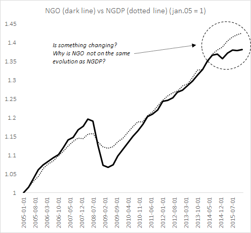
Are we at a new normal point where growth in nominal expenditures is slower than in the past? Yes! But according to Sumner and others, this is 3%. If we use NGO we are much lower! Again, using the FRED dataset, here is the evolution of NGO and NGDP since January 2005 (the start date of the NGO series in a quarterly form). The graph shows something odd starting in mid-2014 : NGO is growing much more slowly.

NGDPNGOaug2016geloso

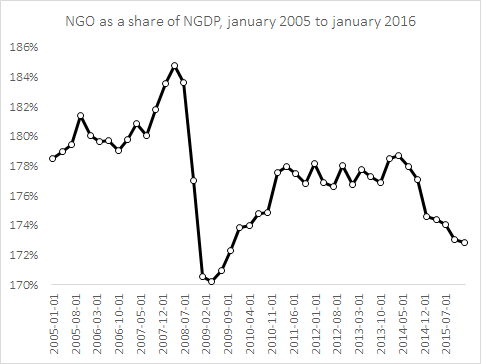
To see this better, let’s plot the evolution of NGO as a percentage of NGDP in the graph below. If the ratio remains stable, then the trend is similar for both. As one can see, the recession saw a much more pronounced fall of NGO than NGDP with a failure to return to the initial levels. And since 2014, the ratio has started to fall again (indicating slower growth of NGO than NGDP).

NGDPoverNGOgeloso2016aug

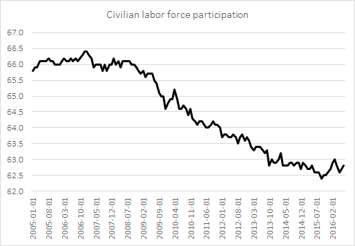
So what is happening? Why is there such a difference? I am not one hundred percent sure about the causes of this difference. However, I am willing to contend that NGO is fitting better than NGDP with other indicators indicating a tepid recovery. If we look at the labor force participation rate in the US, it continues to fall in a nearly mechanical manner. Fewer and fewer workers are at work (or looking for work) in comparison to the population that could be working while investments are disappointing.

CivilianLaborForceParticipation

Maybe Scott Sumner is being overly optimistic. The new trend might simply be substantially lower than he believes.*


*Readers should note that I believe that monetary policy is, at present, too restrictive. However, I believe the culprit is not the Federal Reserve but financial regulations that restrict the circulation of “private money” (the other components of broad money found in divisia indices – see my blog post here). 

Socialism(s) – Part One

Sanders and Me and not so Democratic Socialism

Sen. Sanders got a huge pass this primary season. Captivated by the deep dishonesty of one probable nominee and the crude ignorance of the other (not to mention his plain crudeness), the media, and informal commentators like myself, have not given the Democratic candidate and his program the attention they deserve. Also, in the current primary contest, it’s difficult not to like the guy. I have said several times that he inspires in me a kind of twisted affection. Plus, he has real pluck. But, let’s face it: He is probably done, or done for.

Sen. Sanders has gone very far into the primary while maintaining perfect dignity in his demeanor. He has seldom stooped to personal insults even when he was being severely tried by a Ms Clinton who seems to consider the man’s very candidacy a grave offense, an offense against the natural order of things, a crime of lèse-majesté, even a form of woman abuse. In the meantime Mr Sanders will have single-handedly rehabilitated the word “socialism.” This matters for the future of this nation. Time to look at it critically.

I, personally, especially like Sanders the man. I have reasons to. We are the same age; we went to college at about the same time, both in good universities. He took a fairly active part in the desegregation movement. I did not because it was too early in my American sojourn. (I wish I had taken part.) Nevertheless at age 25, Sanders and I were both leftists. The main difference between us is this: Fifty years later, he has remained impeccably faithful to the ideals of our youth while I walked away, faster and faster, really. I learned to understand the invisible hand of the market. I did some good readings. I was lucky enough to observe my leftists academic colleagues in action at close range early on. Cannily, I observed that the victorious Vietnamese Communist Party did not establish a workers’ paradise in its part of the world. I loathed authoritarianism in any guise. The Senator, meanwhile, spent his honeymoon in the Soviet Union.

When that latter country fell apart and its archives were open, the Senator had nothing to say about the eighty years of mass atrocities they revealed. I am guessing he did not think he had to because he believed in the democratic brand of socialism. It’s hard to tell how much history he knows. (I think that liberals in general are ignorant, including academic liberals. I could tell you stories about them that would raise the hair on the back of your neck.) It does not take much knowledge though to guess that Lenin and the 1916 Bolsheviks did not originally set out deliberately to create a tyranny. Too bad they had to come to power by overthrowing by force of arms a democratically elected government. (See “Kerensky.”) Still, they named the new country “The Union of Socialist Soviet Republics,” and the word “soviet” means “council,” and “republic” means what it means. But, building socialism wasn’t working out; too many people with bad attitudes. So Lenin had to nudge History a little bit with bayonets, with barbed wire, with organized famines and soon, with a bullet to the back of the head of those who stood in the way. The Bolsheviks were forced to choose between socialism and democracy. They chose the former and they got neither. There is no record of Sen. Sanders making any relevant comment. (As always, I am eager to correct my errors.)

It’s less clear whether the Communist Party of China ever had a democratic plan. The unauthorized biography of Mao by his personal doctor reads like a tissue of horrors right from the start. (Dr. Li Zhisui. The Private Life of Chairman Mao, 1994) The Communist Parties of Eastern Europe simply came to power in the wagon train of the Red Army occupying their countries. None of them ever got close to getting there through free elections. The most interesting is the case of East Germany, ruled by a fusion of a native communist party and of preexisting democratic socialist parties. Together, they achieved a fair degree of material success for the East German people yet, they never managed to make do without a police state. Today, Sanders’ backers may not remember or they may not know that the German Democratic Republic, as it was called with a straight face, disappeared overnight. Someone had left a back door open to this paragon of socialist success and the people immediately started voting with their feet by the tens of thousands.

This is all irrelevant, Senator Sanders’ supporters would claim. You are describing a grave perversion of socialism; again, we only want democratic socialism.

During much of my adult life, the ill-defined words “socialism” and “socialist” were used with all kinds of modifiers: “African socialism,” “Arab socialism.” In all cases, the regimes so named led their countries straight to poverty, usually accompanied by official kleptocracy. In India, a really democratic country, the mild Ghandian-Nehruan form of socialism produced deep poverty for two generations including in the large, educated Indian middle class . (Just compare and contrast with un-socialist South Korea which started in 1953, after a devastating war, much poorer than India had been in 1949 when it became independent.) Socialism – whatever that is – is normally the road sign that points toward generalized poverty. Perhaps, this is only the result of a fateful case of reverse magic naming: Call something good, reasonable “socialist” and it begins degrading and sinking! Go figure!

OK, this is all about ancient times, they say. So, let’s look at current examples.

In Venezuela, socialism started under unusually favorable conditions because the country had considerable oil income that minimized the need for high taxation, a major reason for discontent in most socialist experiments. Yet, the socialists in power there made such a mess of it that today, only a few years later, the country suffers about 400% inflation (in 2016). If you had a dollar’s worth of local money there 12 months ago, it now only buys about a quarter’s worth of milk or bread. The skilled middle-class is leaving or trying to. They may return later; or, they may not. If they don’t, it will take a couple of generations at best to rebuild the country’s human capital after the socialist experiment ends.

Note that the sharp drop in world oil prices has affected many countries. It’s only in “Bolivarian” socialist Venezuela that you will see mass exodus and severe shortages of necessities.

In Brazil, The Workers’ Party is in power. The sitting president is a woman whose bona fide, whose socialist credentials are not in question. When she was young, she was imprisoned and even tortured for her belief in socialism, or because she was a guerrilla. (That’s the name for a left-wing terrorist.) She would now be impeached for making up optimistic economic figures for her country, except for the fact that the man constitutionally designated to replace her is also under indictment for corruption. It was bound to happen. The federal government in Brazil eats up 40% of GDP. The huge national oil company, Petrobras is nationalized; it belongs to the government, a favorite socialist arrangement. So oil revenues belong to everyone which means they belong to no one. Why not help myself a little, generations of Brazilian politicians have figured? There are no shareholders to keep tabs and to complain, after all. Socialism and kleptocracy are like father and son.

But, but, you say, those are Third World countries that have not yet recovered from the corrupting influence of colonialism (200 years later). Point well taken. Here is another case I know well, of a socialist country that has not been colonized since about 50 (BC.) France has been under the guiding hand of the French Socialist Party for nearly five years this time around. By the way, France is a democratic country with fair elections and a free press. The Socialists won fair and square. They were in power for 23 of the 35 years since 1981. They largely implemented their program and there were few rollbacks – except by themselves, a few times when they understood the disastrous effects of the reforms they had implemented. I am thinking of a broad de-nationalization of banks in 1981-82. (This is directly relevant to Sen. Sanders’ thinking.)

The French Socialist Party in power never tried to restrict freedom of the press and it did not fill the prisons with its opponents. (Instead, it emptied them hastily of violent criminals, according to its security critics.) By and large, its rule has been quite civilized. There is just that pesky problem of chronic unemployment which never dips much below 10% (25% for the young; sky is the limit if you are young and your name is “Mohamed”). There is also the fact that economic stagnation is now seen as normal by the young. Has been for a couple of generations, now. And then, there is the unbelievable cultural sterility of French society (another story, obviously that I partially tell elsewhere on this blog. Ask me.)

True story: a few months ago, members of the socialist government celebrated loudly. That was because the government office of economic analysis had revised upward its estimate of annual economic growth from GDP: + 0.4% to +0.6% ! (Yes, that’s 6 tenth of one per cent. It’s true that today, in the spring of 2016, it’s at a respectable annual 2% plus.)

“No, no,” cries Sen. Sanders ( and I can almost hear him from here) “I don’t mean ‘socialist’ as in ‘Union of Socialist Soviet Republics,’ and I don’t mean Red China, and I don’t mean North Korea, certainly, and I don’t mean Cuba (although…), and I don’t mean Venezuela today, or Brazil. And, I don’t even mean France although I could not explain why exactly. (Bad call here, Senator. The French single-payer health care system works well; it’s cheaper than US health care, and French men live two years longer than American men.) I mean socialism as in Denmark and Sweden. Now, here we are at last. In part Two, we will look at what passes for Swedish “socialism.” (Denmark is too small to be an example, perhaps.)

A Note on the Econometric Evaluation of Presidents

Sometimes, I feel that some authors simply evolve separately from all those who might be critical of their opinions. I feel that this hurts the discipline of economics since it is better to confront potentially discomforting opinions. And discomforting opinions are never found in intellectually homogeneous groups. However, a recent paper in the American Economic Review by Alan Blinder and Mark Watson suffers exactly from this issue.

Now, don’t get me wrong, the article is highly interesting and provides numerous factoids worth considering when debating economic policy and politics. Basically, the article considers the differences in economic performance under different presidents (and their party affiliation). Overall, it seems that Democrats have a slight edge – but in large part because of “luck” (roughly speaking).

However, no where in the list of references do we find an article to the public choice theory literature. And its not as if that field had nothing to say. There are tons of papers on policy decisions and the form of government. In the AER paper, this can be best seen when Blinder and Watson ask if it was Congress, instead of the president, that caused the differences in performance. That is a correct robustness check, but it is still a mis-specification. There is a strong literature on “divided government” in the field of public choice.

In the case of the United States, this would be presidents and congresses (or even different chambers of congress) of different party affiliation. Generally, government spending is found to grow much more slowly (even relative to GDP) when congress and the White House are held by different parties. Why not extend that conclusion to economic growth? I would not be surprised that lagged values of divided government (mixed partisanships in t minus one) would have a positive on non-lagged growth rates (growth in t-zero).

Now, this criticism is not sufficient to render uninteresting the Blinder-Watson paper. However, it shows that some points fall flat when two fields fail to link together. Public choice theory, in spite of the wide fame of James Buchanan (Nobel 1986), Gordon Tullock and affiliates (or off-spawns) like Elinor Ostrom (Nobel 2009), is still clearly unknown to some in the mainstream.

And that is a disappointment…

The High Wage Economy: the Stephenson critic

A recent trend has emerged in economics. The claim is that high wages can have a dynamic positive effect on market economies.  The intuition is that high wages increase productivity because they incite management to find new techniques of production. In essence, its an argument about efficiency wages: efficiency wages increase incentives to innovate on the part of managers, they can also incite workers to acquire more human capital and work harder and more diligently.

In economic history, this claim has been taken up by scholars like Robert Allen (see his work here for the general public) who argues that the Industrial Revolution took place in England because of high wages. The high-wages of England in the 17th and 18th centuries (relative to all other areas in Europe), together with cheap energy, created an incentive for capital-intensive methods of production (i.e. the industrial revolution). In fact, a great share of the literature on the desirability of high wages for economic development has emanated from the field of economic history.

I have always been skeptical of this argument for two reasons. The first is that efficiency wages is a strange theory that relies on debatable assumptions about labor (strangely, I have been convinced of this point by Austrian scholars like Don Bellante and Pavel Ryksa). The second is that numerous scholars have advanced large criticisms of the underlying data. Robert Allen – the figurehead proponent of the high wage argument – has been constantly criticized by historians like Jane Humphries (see here) for the quality of the data and assumptions used. Allen defends himself on numerous occasions and many of his replies (mainly those on the role of family size in living standards) show that his initial case might have been too conservative (i.e. he is more “correct” than he claims).

Until a year or two ago, I was agnostic on the issue even though I was skeptical. That was until I met Judy Stephenson – a colleague at the London School of Economics. Judy did what I really like to do – dig for data (yes, I am weird like that). She went to the original sources of data used by Allen and others and she looked at what any Law-and-Economics buffs like me like to look at – transaction costs and contracting models.

She recently published her work as a working paper at the LSE and what she found is crucial! Labor was not hired directly, it was hired through contractors who charged costs on the basis of days worked. But this did not translate into wages actually paid to workers. The costs included risks and overheads for contractors. Somewhere between 20% and 30% of the daily costs were not given to workers as wages. Thus, the wage series used to claim that England (Stephenson concentrates on London though) had high wages are actually 20% to 30% below the level often reported. They are also substantially close to those in western Europe.

Thus, the high wage story for England seems weaker. This little piece of historical evidence brought about by Judy is something to think about carefully when one makes the argument that high wages are conducive to growth. Since most of the argument brought to the public was informed largely by this argument in economic history, it makes sense to be cautious when thinking about it in the future.

Can we use tax data to measure living standards (part 2)?

Yesterday, my post on the differences in per capita income and total income per tax unit caused some friends to be puzzled by my results. To their credit, the point can be defended that tax units are not the same as households and the number of tax units may have increased faster than population (example: a father in 1920 filled one tax unit even though his household had six members, but with more single households in the 1960s onwards the number of tax units could rise faster than population for a time).

The problems regarding the use of tax units instead of households is not new. In fact, it is one of the sticking point advanced by skeptics like Alan Reynolds (see his 2006 book) and, more recently, by Richard Burkhauser of Cornell University (see his National Tax Journal article here).

Could it be that all the differences between GDP per person and income per tax unit are caused by this problem? Not really.

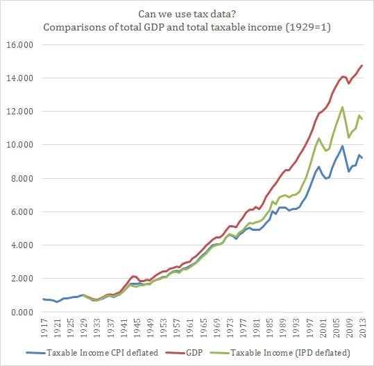
There is an easy to see if the problem is real. Both measures are ratios (income over a population). Either the numerator is wrong or the denominator is wrong. Those who view tax units as the problem argue that the problem is the denominator. I do not agree since I believe that the numerator is at fault. The way to see this is simply to plot total income reported by all tax units and compare this with real GDP. What’s the result?

Even with tax-reported income being deflated with the Implicit Price Deflator (IPD) instead of the consumer price index, we end up with a difference (in 2013) of roughly 3 orders of magnitude between GDP and tax-reported income relative to the 1929 base point. Basically, GDP has increased by a factor of 14.749 since 1929 while IPD-deflated tax-reported income has only increased by a factor of 11.546.

TaxData

As a result, I do not believe that the problem is the tax unit issue. The problem seems to be that tax data is not capturing the same thing as GDP is!

Why farms die and should die


In Canada, I have the frustrating habit of criticizing government support to the agricultural sector especially entry-barriers in the form of production quotas. Most of those policies are regressive in the sense that they reallocate income from the poorest to the richest. In fact, their entire aim is to artificially increase the income of farmers (especially dairy and poultry farmers) at the expense of the rest of the population. However, when lobbyists for these subsidies come out in public, they do so under different disguises. Their favorite? Farms are dying.

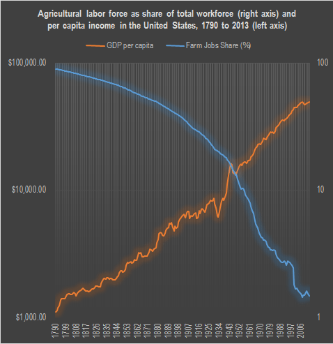
In each radio debate where that boogeyman is raised, I reply that “yes, they are dying and its a good thing”. If we can feed more and more people with less and less farmers using less and less land, that’s a good thing. In fact, it’s the greatest thing that happened in economic history. Less two centuries ago, 90% of the workers in some western economies were involved in agricultural activities. Today, that proportion has fallen to less than 1.5%. Thousands of farms disappeared, we liberated millions of acres of land to return to their natural state and in the process, we became rich and well-fed!

In testimony of this fact, which is my favorite economic history fact, I decided to recompute a graph by Mark Perry of the American Enterprise Institute but I added the GDP per capita figures for the same period (1790 to 2013).

GDPagriculture

Yes, let the farms die. Let the most productive stay in the fields and let them feed humanity while the others become engineers, doctors, teachers, businessmen, welders, carpenters or whatever trade they are best at!

Women and secular stagnation

As an economic historian, I’ve always had a hard time with the idea of secular stagnation. After all, one decade of slow growth is merely a blip on the twelve millenniums of economic history (I am not that interested with the pre-Neolithic history, but there is some great work to be found in archaeology journals). Hence, Robert Gordon’s arguments fall short on me.

That was until I was sparked to react to a comment by Emily Skarbek at Econlib. Overall, she is skeptical of Gordon’s claims of secular stagnation. But not for the same reasons. She claims that there are many improvements in welfare that we are not capturing through national income accounts. This is basically the same point as the one made by the great Joel Mokyr (the gold standard of economic historians).

It is true that national accounts have some large conceptual problems regarding measuring output when there are massive technological changes. Yet, all these problems don’t go in the same direction. More precisely, they don’t all lead to underestimation of growth.

My favorite example of one that leads us to overestimate growth is the one I keep giving my macroeconomics students at HEC Montreal. Assume an economy with a labor-force participation rate of 50%. Basically, only males work. All women stay at home for household chores and childcare. In that case, all measured output is male-produced output. Since national accounts don’t consider household production, all the output of women in the households of this scenario is non-existent.

Now assume a technological change causing a shift of 10% of women to the workforce at the same wage rate as men. That boosts labor participation rate to 55% and output by 5%. However, that would largely overestimate growth caused by this shift. After all, when my grandmothers were raising my parents, they were producing something. It was not worthless output. Obviously, if my grandmothers went to work, there was some net added value, but not as much as 5%. However, according to national account, the net increase in GDP is … 5%.

Obviously wrong right? Now, think of the economic history of the last 100 years. Progressively, female labor-force participation increased as marriages were delayed and family sizes were reduced. Unmarried women stayed on the market longer. Then, the introduction of new household technologies allowed some married women to join the labor force more actively. Progressively, women accumulated more human capital and became more active in the labor force. So much that in many western countries, both genders have equal labor-force participation rates.

As they shifted from household production to market production, we considered that everything they did was a net added value. We never subtracted the value of what was produced before. Don’t get me wrong, I am happy that women work instead of toiling inside a household to handwash dirty clothes. Yet, it would be both statistically incorrect and morally insulting to say that what women did in the household had no value whatsoever. 

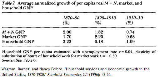
The role of household production in reducing the quality of growth estimates goes back to the 1870s! A 1996 article in Feminist Economics (which I use a lot in my own national account sections of macroeconomics classes) shows the following changes in growth rates when we account for the value of household production. Instead of increasing to 1910 and then falling to 1930, growth in the United States falls to 1930. While the growth rates remain appreciable, they nonetheless indicate a massively different interpretation of American economic history.

SecularStagnation


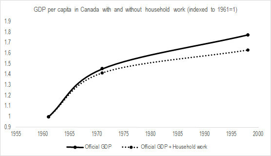
Sadly, I do not possess a continuation of such estimates to later points in time for the United States. I know there is an article by the brilliant Valerie Ramey in the Journal of Economic History, but I am not sure how to compute this to reflect changes in overall output. I intend to try to find them for a short piece I want to submit later in 2016. Yet, I do have estimates for my home country of Canada. Combining a 1979 paper in the Review of Income and Wealth with a working paper from Statistics Canada, it seems that the value of household production falls from 45% of GNP in 1961 to 33% in 1998. When we adjust GDP per capita to consider the changes in household work in Canada, the growth path remains positive, but it is less impressive.

SEcularStagnation2

I am not saying that Gordon is right to say that growth is over. I am saying that the accounting problems don’t all go in the direction of invalidating him. In fact, if my point is correct, proper corrections would reduce growth rates dramatically for the period of 1945 to 1975 and less so for the period that followed. This may indicate that “slow growth” was with us for most of the post-war era. That’s why I reacted to the blog post of Skarbek.

It also allows me to say the thing that is the best buzz-kill for economics students: national accounting matters!

Malthusian pressures (as outcome of rent-seeking)

Nearly a week ago, I intervened in a debate between Anton Howes of King’s College London whose work I have been secretly following  (I say “secretly” because as an alumnus of the London School of Economics, I am not allowed to show respect for someone of King’s College) and Pseudoerasmus (whose identity is unknown but whose posts are always very erudite and of high quality – let’s hope I did not just write that about an alumnus of King’s College). Both bloggers are heavily involved in my first field of interest – economic history.

The debate concerned the “Smithian” counter-effect to “Malthusian pressures”. The latter concept refers to the idea that, absent technological innovation,  population growth will lead to declining per capita as a result of marginally declining returns. The former refers to the advantages of larger populations: economies of scale, more scope for specialization and market integration thanks to density. Now, let me state outright that I think people misunderstand Malthusian pressures and the Smithian counter-effect.

My point of is that both the “Smithian counter-effect” and “Malthusian pressures” are merely symptoms of rent-seeking or coordination failures. In the presence of strong rent-seeking by actors seeking to reduce competition, the Smithian counter-effect wavers and Malthus has the upper hand. Either through de-specialization, thinner of markets, shifting to labor-intensive technologies, market disintegration and lower economies of scale, rent-seeking diminishes the A in a classical Cobb-Douglas function of Total Factor Productivity (Y=AKL). This insight is derived from my reading of the article by Lewis Davis in the Journal of Economic Behavior and Organization which contends that “scale effects” (another name for a slight variant of the “Smithian counter-effect) are determined by transaction costs which are in turn determined by institutions. If institutions tend to favor rent-seeking, they will increase the likelihood of coordination failure. It is only then that coordination failures will lead to “Malthusian pressures” with little “Smithian counter-effect”. Institutions whose rules discourage rent-seeking will allow markets to better coordinate resource use so as to maximize the strength of the “Smithian counter-effect” while minimizing the dismal Malthusian pressures.

In essence, I don’t see the issue as one of demography, but as one of institutions, public choice and governance. I am not alone in seeing it this way (Julian Simon, Jane Jacobs and Ester Boserup have documented this well before I did). Why the divergence?

This is because many individuals misunderstand what “Malthusian pressures” are. In an article I published in the Journal of Population Research, me and Vadim Kufenko summarize the Malthusian model as a “general equilibrium model”. In the long run, there is an equilibrium level of population with a given technological setting. In short-run, however, population responds to variation in real wages. Higher real wages from a “temporary” positive real shock will lead to more babies. However, once the shock fades, population will adapt through two checks: the preventive check and the positive check. The preventive check refers to households delaying family formation. This may be expressed through later marriage ages, planned sexual activities, contraception, longer stays in the parental household and greater spacing between births. The positive check refers to the impact of mortality increasing to force the population back to equilibrium level. These checks return to the long-term equilibrium. Hence, when people think of “Malthusian pressures”, they think of population growth continuing unchecked with scarce ressources. But the “Malthusian model” is basically a general equilibrium model of population under fixed technology. In that model, there are no pressures since the equilibrium rates of births and deaths are constant (at equilibrium).

However, with my viewpoint, the equilibrium levels move frequently as a result of institutional regimes. They determine the level of deaths and births. “Poor” institutions will lead to more frequent coordination failures which may cause, for a time, population to be above equilibrium – forcing an adjustment. “Poor” institutions would also lead to an inability to respond to a change in constraints (i.e. the immediate environment) by being rigid or stuck with path-depedency problems which would also imply the need for an adjustment.  “Good” institutions will allow “the Smithian counter-effect” to intervene through arbitrage across markets to smooth the effect of local shocks, a greater scope for specialization etc.

My best case for illustration is a working paper I have with Vadim Kufenko (University of Hohenheim) and Alex Arsenault Morin (HEC Montréal) where we argue that population pressures as exhibited by the very high levels of infant mortality rates in mid-19th century Quebec were the result of institutional regimes. The system of land tenure for the vast majority of the population of Quebec was “seigneurial” and implied numerous regressive transfers and monopoly rights for landlords. This system was also associated with numerous restrictions on mobility which limited the ability of peasants to defect and move. However, a minority of the population (but a growing one) lived under a different institution which did not impose such restrictions, duties and monopolies. In these areas, infant mortality was considerably lower. We find that, adjusting for land quality and other factors, infant mortality was lower in these areas for most age groups. Hence, we argued that what was long considered as “Malthusian pressures” were in fact “institutional pressures”.

Hence, when I hear people saying that there are problems linked to “growing population”, I hear “because institutions make this a problem” (i.e. rent seeking).

Was Murphy Foolish to Take Caplan’s Bet?

A few days ago, Bryan Caplan posted on his bet with Robert Murphy regarding inflation. Murphy predicted 10% inflation. He lost … big time. However, was he crazy to make that bet?  In other words, what could explain Caplan’s victory?

Murphy was not alone in predicting this, I distinctly remember a podcast between Russ Roberts and Joshua Angrist on this where Roberts tells Angrist he expected high inflation back in 2008. Their claims were not indefensible. Central banks were engaging in quantitative easing and there was an important increase of the state money supply. There was a case to be made that inflation could surge.

It did not. Why?

In a tweet, Caplan tells me that monetary transmission channels are much more complex than they used to be and that the TIPS market knew this. Although I agree with both these points, it does not really explain why it did not materialize. I am going to propose two possibilities of which I am not fully convinced myself but whose possibility I cannot dismiss out of hand.

Imagine an AS-AD graph. If Murphy had been right, we should have seen aggregate demand stimulated to a point well above that of long-run equilibrium. Yet, its hard to see how quantitative easing did not somehow stimulate aggregate demand.  Now, if aggregate demand was falling and that quantitative easing merely prevented it from falling, this is what would prove Murphy wrong. However, all of this assumes no movement of supply curves.

While AD falls and before monetary policy kicks in, imagine that policies are adopted that reduce the potential for growth and productivity improvement. In a way, this would be the argument brought forward by people like Casey Mulligan in work on labor supply and the “redistribution recession” and Edward Prescott and Ellen McGrattan who argue that, once you account for intangible capital, the real business cycle model is still in play (there was a TFP shock somehow). This case would mean that as AD fell, AS fell with it. I would find it hard to imagine that AS shifted left faster than AD. However, a relatively smaller fall of AS would lead to a strong recession without much deflation (which is what we have seen in this recession). Personally, I think there is some evidence for that. After all, we keep reducing the estimate for potential GDP everywhere while the policy uncertainty index proposed by Baker, Bloom and Davids shows a level change around 2008.  Furthermore, there has been a wave – in my opinion of very harmful regulations – which would have created a maze of administrative costs to deal with (and whose burden is heavy according to Dawson and Seater in the Journal of Economic Growth). That could be one possibility that would explain why Murphy lost.

download

There is a second possibility worth considering (and one which I find more appealing): the role of financial regulations. Now, I may have been trained mostly by Real Business Cycle guys, but I do have a strong monetarist bent. I have always been convinced by the arguments of Steve Hanke and Tim Congdon (I especially link Congdon) and others that what you should care about is not M1 or M2, but “broad money”. As Hanke keeps pointing out, only a share of everything that we could qualify broadly as “money” is actually “state money”. The rest is “private money”. If a wave of financial regulations discourages banks to lend or incite them to keep greater reserves, this would be the equivalent of a drop of the money multiplier. If those regulations are enacted at the same time as monetary authorities are trying to offset a fall in aggregate demand, then the result depends on the relative impact of the regulations. The data for “broad money” (Hanke defines it as M4) shows convincingly that this is a potent contender. In that case, Murphy’s only error would have been to assume that the Federal Reserve’s policy took place with everything else being equal (which was not the case since everything seemed to be moving in confusing directions).

globr-asia-nov-2014-1bg

In the end, I think all of these explanations have value (a real shock, a banking regulation shock, an aggregate demand shock). In 25 years when economic historians such as myself will study the “Great Recession”, they will be forced to do like they do with Great Depression: tell a multifaceted story of intermingled causes and counter-effects for which no single statistical test can be designed. When cases like these emerge, it’s hard to tell what is happening and those who are willing to bet are daredevils.

P.S. I have seen the blog posts by Scott Sumner and Marcus Nunes regarding my NGO /NGDP claims. They make very valid points and I want to take decent time to address them, especially since I am using the blogging conversation as a tool to shape a working paper.