The High Wage Economy: the Stephenson critic

A recent trend has emerged in economics. The claim is that high wages can have a dynamic positive effect on market economies.  The intuition is that high wages increase productivity because they incite management to find new techniques of production. In essence, its an argument about efficiency wages: efficiency wages increase incentives to innovate on the part of managers, they can also incite workers to acquire more human capital and work harder and more diligently.

In economic history, this claim has been taken up by scholars like Robert Allen (see his work here for the general public) who argues that the Industrial Revolution took place in England because of high wages. The high-wages of England in the 17th and 18th centuries (relative to all other areas in Europe), together with cheap energy, created an incentive for capital-intensive methods of production (i.e. the industrial revolution). In fact, a great share of the literature on the desirability of high wages for economic development has emanated from the field of economic history.

I have always been skeptical of this argument for two reasons. The first is that efficiency wages is a strange theory that relies on debatable assumptions about labor (strangely, I have been convinced of this point by Austrian scholars like Don Bellante and Pavel Ryksa). The second is that numerous scholars have advanced large criticisms of the underlying data. Robert Allen – the figurehead proponent of the high wage argument – has been constantly criticized by historians like Jane Humphries (see here) for the quality of the data and assumptions used. Allen defends himself on numerous occasions and many of his replies (mainly those on the role of family size in living standards) show that his initial case might have been too conservative (i.e. he is more “correct” than he claims).

Until a year or two ago, I was agnostic on the issue even though I was skeptical. That was until I met Judy Stephenson – a colleague at the London School of Economics. Judy did what I really like to do – dig for data (yes, I am weird like that). She went to the original sources of data used by Allen and others and she looked at what any Law-and-Economics buffs like me like to look at – transaction costs and contracting models.

She recently published her work as a working paper at the LSE and what she found is crucial! Labor was not hired directly, it was hired through contractors who charged costs on the basis of days worked. But this did not translate into wages actually paid to workers. The costs included risks and overheads for contractors. Somewhere between 20% and 30% of the daily costs were not given to workers as wages. Thus, the wage series used to claim that England (Stephenson concentrates on London though) had high wages are actually 20% to 30% below the level often reported. They are also substantially close to those in western Europe.

Thus, the high wage story for England seems weaker. This little piece of historical evidence brought about by Judy is something to think about carefully when one makes the argument that high wages are conducive to growth. Since most of the argument brought to the public was informed largely by this argument in economic history, it makes sense to be cautious when thinking about it in the future.

On the Canadian economy: the “real” problem

In Canada, the state of the economy has everyone worried. The fall in oil prices is causing the oil sector in the western provinces and in some of the Atlantic provinces to contract. As a result, everyone has the impression that Canada is sliding towards a recession and governments should act.

I disagree. My disagreement is fueled by two factors. The first is that we should never reason from a price change. The fall in the price of oil is mostly the result of increasing supply of oil. Such a price change is actually a good thing for the Canadian economy. The slowdown in economic activity is merely the result of frictions in the reallocation of resources. The second reason is that the slowdown is caused by “real factors” – policy decision affecting key regions of the Canadian economy. Any government action would worsen a situation caused by too much interference in the first place.

A fall in oil prices can indeed affect the Canadian economy. The oil produced in Canada is generally profitable when prices are relatively high (they require very capital-intensive methods of extraction and refining). An increase in the world oil supply (which is the case right now) would indeed affect the Canadian oil industry. However, Canadians win through lower oil prices – one important input has gotten cheaper. The problem is that once such a slowdown happens, resources are not reallocated without frictions. Business plans are positively affected by the lower oil prices and numerous firms are laying out new plans to expand production. Employment and output will fall in the oil industry before they will pick up in other industries. Eventually, there might even be greater output and employment because of the greater worldwide supply of oil. Right now, Canada is in-between those two situations.

My second reason for dissenting from the majority opinion is that certain regions of the Canadian economy are plagued by poor policy. To make my argument, consider a two-region (West and East) and two-industry economy (oil and manufacturing/services). In the West, the dominant industry is oil. In the East, the dominant industry is manufacturing/services.  The West economy has a more flexible market for inputs (limited regulation, freer labor market and low taxes on capital). The East economy suffers from greater rigidity in its market for inputs – high taxes, burdensome regulation and stringent labor laws.

In a way, this describes the Canadian economy. The provinces of Alberta, Saskatchewan, Manitoba and British-Columbia have been pulling the rest of the Canadian economy for the last twenty years. That’s the West. In the East, the historically poorer province of Quebec has been constantly pulling everyone behind, but less so in recent years as the province of Ontario (the most populous of Canadian provinces) began to slow down. Ontario dramatically expanded the size of its public sector, implemented important regulations and raised taxes – straight in the middle of the recession. In fact, if you exclude Ontario from the rest of Canada, you find (as Philip Cross did) that Canada’s performance is actually quite decent. So in the East, you have Quebec whose policies have not changed and you have Ontario who has adopted increasingly anti-growth policies. The East also has consistently higher taxes. The West has lower taxes. Etc.

Given the accuracy of this stylized description, imagine the effect of a shock on the western economy through a shock on its oil industry. Normally, firms in the East could adapt to lower oil prices by expanding their output in the manufacturing/services sector (thanks to cheaper inputs) while firms in the West contract their output and liberate inputs. However, in the presence of government-imposed frictions, this reallocation of resources is much harder and output has a harder time expanding in the East.

No demand-side policy can solve this problem! You could have easy money and a massive stimulus program, but if firms are discouraged from increasing output, little will happen. In Canada, the current slowdown is explained by “real factors”. Improving provincial policies would be the best channel for improving the state of the Canadian economy.

Can we use tax data to measure living standards (part 2)?

Yesterday, my post on the differences in per capita income and total income per tax unit caused some friends to be puzzled by my results. To their credit, the point can be defended that tax units are not the same as households and the number of tax units may have increased faster than population (example: a father in 1920 filled one tax unit even though his household had six members, but with more single households in the 1960s onwards the number of tax units could rise faster than population for a time).

The problems regarding the use of tax units instead of households is not new. In fact, it is one of the sticking point advanced by skeptics like Alan Reynolds (see his 2006 book) and, more recently, by Richard Burkhauser of Cornell University (see his National Tax Journal article here).

Could it be that all the differences between GDP per person and income per tax unit are caused by this problem? Not really.

There is an easy to see if the problem is real. Both measures are ratios (income over a population). Either the numerator is wrong or the denominator is wrong. Those who view tax units as the problem argue that the problem is the denominator. I do not agree since I believe that the numerator is at fault. The way to see this is simply to plot total income reported by all tax units and compare this with real GDP. What’s the result?

Even with tax-reported income being deflated with the Implicit Price Deflator (IPD) instead of the consumer price index, we end up with a difference (in 2013) of roughly 3 orders of magnitude between GDP and tax-reported income relative to the 1929 base point. Basically, GDP has increased by a factor of 14.749 since 1929 while IPD-deflated tax-reported income has only increased by a factor of 11.546.

TaxData

As a result, I do not believe that the problem is the tax unit issue. The problem seems to be that tax data is not capturing the same thing as GDP is!

Can we use tax units to measure living standards?

In the debate on inequality, I am a skeptic of how large a problem the issue is. Personally, I tend to believe that worries of inequality only increase when growth is stagnant. In fact, I also believe that there are numerous statistical biases causing us to misidentify stagnation as rising inequality. Most of the debate on inequality is plagued with statistical problems of daunting magnitudes (regional convergence in income, regional price levels, demographic changes, increasing heterogeneity of preferences, increasing heterogeneity of personal characteristics, income not being purely monetary, the role of taxes and transfers etc.)

One of them centers around the use of tax data. This has been the domain of Thomas Piketty and Emmanuel Saez. I can understand the appeal of using tax data since it is easily available and usable. Yet, is it perfect?

A year or two ago, I would have been inclined to simply say “yes” and not bother with the details. Theoretically, taxes should be an “okay” proxy for the income distribution and should follow average income even if at different levels. Yet, after reading the article of Phil Magness and Robert Murphy in the Journal of Private Enterprise I confess that I am no longer accepting anything as “granted” in the inequality debate. So, I simply decided to chart GDP per capita with the average taxable income per tax unit. Just to see what happens. Both are basically averages of the overall population, they should look pretty much the same (theoretically).  The data for the tax units is made available in the Mark W. Frank dataset based on the Piketty-Saez data (see here) and I deflated with both the CPI and the implicit price deflator available at FRED/St-Louis.

The result is the following and it shows two very different stories! Either the GDP statistics are wrong and we have average stagnation (which does not mean that there is no increase in inequality) or the taxable income data is wrong in estimating the trend of living standards and the GDP are closer to reality (which does not that there is no increase in inequality).  In the end, there is a problem to be assessed with the quality of the data used to measure inequality.

Tax Data

Down All Your Markets

The US stock market had its worst ever initial trading weeks in 2016. Speculators are alarmed by the fall in the stocks of China. The economy of China has been growing more slowly, if at all. Also, most of the economies of the world are in growth recessions, a reduction in the rate of growth. The US dollar is high relative to other currencies, which reduces exports.

The government of China has yet to learn that interventions into financial markets often backfire. The Chinese chiefs have halted stock transactions when the market average falls to seven percent. They also have not allowed sales by investors who own more than five percent of a company. One problem with financial “circuit breakers” – a halt of trading – is that when stocks start to fall, speculators will panic and sell more quickly before trading halts. Restrictions on selling stocks create uncertainty when buying them. A speculator will fear being unable to sell shares later.

There is enough inherent uncertainty in markets without government adding to it. Uncertainty makes it important to let the market set the prices. Markets are a discovery process in which prices and quantities evolve through the bids of buyers and offers of sellers. When government interferes, we cannot know the price. Since the leaders of China have decided to have a market economy in goods, input factors, and financial assets, they should allow the market to do its job of setting the prices.

When I visited China three times, I saw a forest of cranes in all the cities I went to. Construction has driven the economy of China, along with exports. But, similar to real estate booms elsewhere, this construction was propelled by governmental policy. Throughout the world, cheap credit and fiscal subsidies to real estate have fueled unsustainable speculation.

Now China has much excess building capacity, and the halt in construction reduces related goods such as furniture and raw materials. The slow-down in China and sluggish growth elsewhere has resulted in a collapse of commodity prices.

The chiefs of China seek to move the country’s economy towards more domestic consumption. But they interfere with domestic spending by imposing a value-added tax of 17 percent on most goods other than real estate. The government of China probably chose to impose a VAT because the World Trade Organization allows the VAT to be subtracted from the price of exports, unlike an income tax. But Chinese consumers suffer a higher cost of living.

The Chinese leaders could have instead enacted LVT, land-value taxation, which would not add to the cost of goods. A tax on land value reduces the purchase price but not the land rent, so also not the price of goods. A tax on most of the rent or land value would stop the land speculation that has made a few people rich at the expense of the public.

The government of China still maintains tight control over the banking system. All the markets – real estate, financial, goods – would be more efficient if interest rates too were set by the market supply and demand for loanable funds. Of course the central banks of Europe, Japan, and the USA also are not letting their markets set the money supply and interest rates. But common practice does not imply optimal policy.

I don’t think the big drop in stock market averages imply impending economic doom. For 200 years, the US economy has had a real estate cycle of an average duration of 18 years. The current cycle began with the depression of 2008. The recovery has been slow, but the expansion has continued as employment and output have grown. Real estate construction has contributed to the expansion, and land values have recovered. The economy seldom has a recession while interest rates and commodity prices are low.

The economy of China has some severe long-run problems, but its economy is still developing and catching up. The government seems ready to let the currency trade more freely, and the coming acceptance of the currency (the yuan or renminbi) into the “special drawing rights” of the International Monetary Fund will boost the economy.

In the short run, the US stock market could fall some more, as markets often overreach, but over the next few years, financial markets will be consistent with the economic reality of restored world-wide economic growth, if there are no major destructive attacks. What we should be worried about is the unsustainability of debt and the next real estate speculative boom. The next economic disaster is about a decade into the future, and nobody is yet alarmed about that.

NGO v. NGDP: In reply to Nunes and Sumner

A week ago, I initiated a discussion on using another indicator of nominal spending instead of NGDP when the time comes to set monetary policy. My claim was that NGDP includes only final goods and as a result, it misses numerous business-to-business transactions. This means that NGDP would not be the best indicator. I propose a shift to a measure that would capture some intermediate transactions.

The result was a response by Nick Rowe (to which I did respond), Matt Rognlie, Marcus Nunes and Scott Sumner (to whom I am responding now). Nunes and Sumner are particularly skeptical of my claim. I am providing a first response here (and I am attempting to expand it for a working paper).

The case against NGDP

GDP has important shortcomings. First of all, thanks to the work of Prescott and McGrattan (2012 : 115-154), we know that a sizable part of capital goods acquisition fails to be included inside GDP. That sizable part is “intangible capital” which Prescott and McGrattan define as the “accumulated know-how from investing in research and development, brands, and organizations which is the most part expensed rather than capitalized” (p.116).  Yet, investments in research and development are – in pure theoretical terms – like the acquisition of capital goods. However, national accounts exclude those. Once they’re included in papers like those of Prescott and McGrattan and those of Corrado, Hulten and Sichel (2009), increases in productivity were faster prior to 2008 and that the collapse after 2008 was much more pronounced.  In addition, this form of capital is increasing much faster than tangible so that its share of the total capital stock increases. Thus, the error of not capturing this form of capital good investment is actually growing over time causing us to miss both the level and the trend.

A second shortcoming of importance is the role of time in production. Now, just the utterance of these words makes me sound like an Austrian. Yet, this point is very neoclassical since it relies on the time to build approach. In the time-to-build model of the real business cycle approach, production occurs over many periods. Thus changes in monetary policy may have some persistence.  The time-to-build model proposes that firms undertake long projects and consume more inputs. In terms of overall transactions, this will mean more and more business to business (B2B) transactions.  Hence if an easy monetary policy is inciting individuals to expand their number of projects that have more distant maturities, then a focus on GDP won’t capture the distortionary effects of that policy through. Similarly, if monetary policy tightens (either directly as a fall of the money supply or through an uncompensated change in velocity), the drop in economic activity as projects are closed down will not equally well captured. While this point was initially advanced by Kyland and Prescott (1982), some Austrians economists have taken up the issue (Montgomery 1995a; 1995b; 2006; Wainhouse 1984; Mulligan 2010), several neoclassicals have also taken it up (Kühn 2007; Kalouptsidi 2014; Kyland, Rupert, Sustek, 2014).

Why shift to another measure

My contention is that NGO (Nominal Gross Output) allows us to solve a part of that problem. First of all, NGO is more likely to capture a large share of the intangible capital part since, as a statistic, it does not concern itself with double counting. Hence, most of the intangible capital expenses are captured. Secondly, it also captures the time-to-build problem by virtue of capturing inputs being reallocated to the production of projects with longer maturities.

Thus, NGO is a better option because it it tries to capture the structure of production. The intangible capital problem and the time to build problem are both problems of intermediate goods. By capturing those, we get a better approximate idea of the demand for money.

Let me argue my case based on the Yeager-esque assumption that any monetary disequilibrium is a discrepancy between actual and desired money holdings at a given price level. Let me also state the importance of the Cantillon effects whereby the point of entry of money is important.

If an injection of money is made through a given sector that leads him to expand his output, the reliability of NGDP will be best if the entry-point predominantly affects final goods industry. If it enters through a sector which desires to spend more on intangible investments or undertake long-term projects, then the effects of that change will not appear as they will merely go unmeasured. They will nonetheless exist. Eventually firms will realize that they took credit for these projects for which the increased output did not meet any demand. The result is that they have to contract their output by a sizable margin. In that case, they will abandon those activities (imagine unfinished skyscrapers or jettisoned research projects).

In such situations, GO (or even a wider measure of gross domestic expenditures) are superior to GDP. And in cases where the effects would start in final-goods industry, then they have the same efficiency as GO (or the wider measure of gross domestic expenditures.

The empirical case

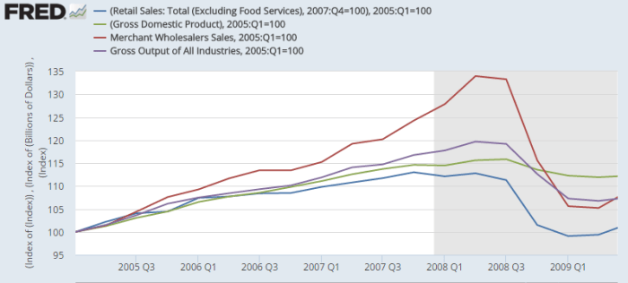
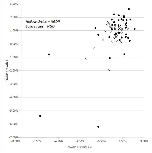
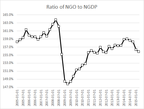
The recurring criticism in most posts is that NGO is volatile over the period when the data is available (2005Q1-today). True, the average growth rate of NGO is the same as NGDP over the same period, but the standard deviation is nearly twice that of NGDP. However if you exclude the initial shock of the recession, the standard deviations converge. In a way, all the difference in volatility between the two series is driven by the shock of the recession. Another way to see it is to recompute two graphs. One is an imitation of the graphs by Nunes where NGDP growth in period T is compared with growth in the period T minus 1, but we add NGO. The second is the ratio of NGO to NGDP.

As one can see from the first figure, NGO and NGDP show the same relation except for a cluster of points at the bottom for NGO. All of those lower points are related to the drop from the initial recession. All concentrated at the bottom. This suggests that the recession had a much deeper effect than otherwise believed. The second graph allows us to see it.

Nunes

The ratio of NGO to NGDP shows that the two evolved roughly the same way over the period before the recession. However, when the recession hit, the drop was more important and the ratio never recovered!  This suggest a much deeper deviation from the long-term trend of nominal spending which is not seen at the final level but would be seen rather in the undertaking of long-term projects and the formation of intangible capital (the areas that NGDP cannot easily capture).

Ratio.png

The case for NGO over NGDP is solid. It does not alter the validity of the case for nominal spending stability. However since the case for nominal spending stability hinges on total transactions of inputs and outputs more than it does on the final goods sold, NGO is a better option.


Quick comment in response to Rognlie 
In his reply to Nick Rowe, Matt Rognlie states that the more important fall of NGO is explained by changes in relative prices. Although his transformation shows this, the BEA disagrees. Here is the explanation provided by the BEA:
For example, value added for durable-goods manufacturing dropped 15 percent in 2009, while gross output dropped 19 percent.  The decline in gross output is much more pronounced than the decline in value added because it includes each of the successive declines in the intermediate inputs supply chain required to manufacture the durable goods.


Why farms die and should die


In Canada, I have the frustrating habit of criticizing government support to the agricultural sector especially entry-barriers in the form of production quotas. Most of those policies are regressive in the sense that they reallocate income from the poorest to the richest. In fact, their entire aim is to artificially increase the income of farmers (especially dairy and poultry farmers) at the expense of the rest of the population. However, when lobbyists for these subsidies come out in public, they do so under different disguises. Their favorite? Farms are dying.

In each radio debate where that boogeyman is raised, I reply that “yes, they are dying and its a good thing”. If we can feed more and more people with less and less farmers using less and less land, that’s a good thing. In fact, it’s the greatest thing that happened in economic history. Less two centuries ago, 90% of the workers in some western economies were involved in agricultural activities. Today, that proportion has fallen to less than 1.5%. Thousands of farms disappeared, we liberated millions of acres of land to return to their natural state and in the process, we became rich and well-fed!

In testimony of this fact, which is my favorite economic history fact, I decided to recompute a graph by Mark Perry of the American Enterprise Institute but I added the GDP per capita figures for the same period (1790 to 2013).

GDPagriculture

Yes, let the farms die. Let the most productive stay in the fields and let them feed humanity while the others become engineers, doctors, teachers, businessmen, welders, carpenters or whatever trade they are best at!

Basic income: a debate where demand magically disappears!

For a few months now, the case for the basic income has resurged (I thought it died with Milton Friedman in 2006, if not earlier). In the wake of this debate, I have been stunned by the level of disconnect between the pundits and what the outcome of the few experiments of basic income have been. The most egregious illustration of this disconnect is the case of the work disincentive.

To be clear, most of the studies find a minor effect on labor supply overall which in itself does not seem dramatic (see Robert Moffitt’s work here). Yet, this is a incomplete way to reflect on the equilibrium effect of a massive reform that would be a basic income.

Personally, I think that there is a good reason to believe that the labor supply reaction would be limited. At present, many tax systems have”bubbles” of increasing marginal tax rates. In some countries like Canada, the phasing out of tax credits for children actually mean that the effective marginal tax rate increases as income increases from the low 20,000$ to the mid 40,000$. As a result, a basic income would flatten the marginal tax rate for those whose labor supply curve is not likely to bend backward. In such a situation, labor supply could actually increase!

Yet, even if that point was wrong, labor supply could shift but without any changes in total labor provided. Under most basic income proposals, tax rates are dropped significantly as a result of a reduced bureaucracy and of a unified tax base (i.e. the elimination of tax credits). In such a situation, marginal tax rates are also lowered. This means greater incentives to invest (save) and acquire human capital. This will affect the demand for labor!

A paper in the Journal of Socio-Economics by  Karl Widerquist makes this crucial point. None of the experiments actually could estimate the demand-side reaction of the market. Obviously, a very inelastic labor demand would mean very little change in hours worked and the reverse if it was very elastic. But what happens if the demand curve shifts? Widerquist does not elaborate on shifts of the demand curve, but they could easily occur if a basic income consolidates all transfers (in kind and conditional monetary) allows a reduction in overall spending and thus the tax take needed to fund activities. In that case, demand for labor would shift to the right. A paper on the health effects of MINCOME in Manitoba (Canada) shows that improvement in health outcomes are cheaply attained through basic income which would entail substantial health care expenditures reduction.

I have surveyed the articles compiled by Widerquist and added those who have emerged since. None consider the possibility of a shift of the demand curve. Even libertarian scholars like Matt Zwolinski (who has been making the case forcibly for a basic income for sometime now) have not made this rebuttal point!

Yet, the case is relatively straightforward: current transfers are inefficient, basic income is more efficient at obtaining each unit of poverty reduction, basic income requires lower taxes, basic income means lower marginal tax rates, lower marginal tax rates mean more demand for investment and labor and thus more long-term growth and a counter-balance to any supply-side effect.

I hope that the Bleeding Heart Libertarians will take notice of this crucial point in favor of their argument!

Women and secular stagnation

As an economic historian, I’ve always had a hard time with the idea of secular stagnation. After all, one decade of slow growth is merely a blip on the twelve millenniums of economic history (I am not that interested with the pre-Neolithic history, but there is some great work to be found in archaeology journals). Hence, Robert Gordon’s arguments fall short on me.

That was until I was sparked to react to a comment by Emily Skarbek at Econlib. Overall, she is skeptical of Gordon’s claims of secular stagnation. But not for the same reasons. She claims that there are many improvements in welfare that we are not capturing through national income accounts. This is basically the same point as the one made by the great Joel Mokyr (the gold standard of economic historians).

It is true that national accounts have some large conceptual problems regarding measuring output when there are massive technological changes. Yet, all these problems don’t go in the same direction. More precisely, they don’t all lead to underestimation of growth.

My favorite example of one that leads us to overestimate growth is the one I keep giving my macroeconomics students at HEC Montreal. Assume an economy with a labor-force participation rate of 50%. Basically, only males work. All women stay at home for household chores and childcare. In that case, all measured output is male-produced output. Since national accounts don’t consider household production, all the output of women in the households of this scenario is non-existent.

Now assume a technological change causing a shift of 10% of women to the workforce at the same wage rate as men. That boosts labor participation rate to 55% and output by 5%. However, that would largely overestimate growth caused by this shift. After all, when my grandmothers were raising my parents, they were producing something. It was not worthless output. Obviously, if my grandmothers went to work, there was some net added value, but not as much as 5%. However, according to national account, the net increase in GDP is … 5%.

Obviously wrong right? Now, think of the economic history of the last 100 years. Progressively, female labor-force participation increased as marriages were delayed and family sizes were reduced. Unmarried women stayed on the market longer. Then, the introduction of new household technologies allowed some married women to join the labor force more actively. Progressively, women accumulated more human capital and became more active in the labor force. So much that in many western countries, both genders have equal labor-force participation rates.

As they shifted from household production to market production, we considered that everything they did was a net added value. We never subtracted the value of what was produced before. Don’t get me wrong, I am happy that women work instead of toiling inside a household to handwash dirty clothes. Yet, it would be both statistically incorrect and morally insulting to say that what women did in the household had no value whatsoever. 

The role of household production in reducing the quality of growth estimates goes back to the 1870s! A 1996 article in Feminist Economics (which I use a lot in my own national account sections of macroeconomics classes) shows the following changes in growth rates when we account for the value of household production. Instead of increasing to 1910 and then falling to 1930, growth in the United States falls to 1930. While the growth rates remain appreciable, they nonetheless indicate a massively different interpretation of American economic history.

SecularStagnation


Sadly, I do not possess a continuation of such estimates to later points in time for the United States. I know there is an article by the brilliant Valerie Ramey in the Journal of Economic History, but I am not sure how to compute this to reflect changes in overall output. I intend to try to find them for a short piece I want to submit later in 2016. Yet, I do have estimates for my home country of Canada. Combining a 1979 paper in the Review of Income and Wealth with a working paper from Statistics Canada, it seems that the value of household production falls from 45% of GNP in 1961 to 33% in 1998. When we adjust GDP per capita to consider the changes in household work in Canada, the growth path remains positive, but it is less impressive.

SEcularStagnation2

I am not saying that Gordon is right to say that growth is over. I am saying that the accounting problems don’t all go in the direction of invalidating him. In fact, if my point is correct, proper corrections would reduce growth rates dramatically for the period of 1945 to 1975 and less so for the period that followed. This may indicate that “slow growth” was with us for most of the post-war era. That’s why I reacted to the blog post of Skarbek.

It also allows me to say the thing that is the best buzz-kill for economics students: national accounting matters!

Of Uber, cab drivers and compensation

What a title for a blog post right? Where am I going with this? A few days ago, I debated a few of my academic colleagues who tend towards libertarianism in the predominantly left-leaning province of Quebec. The topic? How the rise of Uber is killing the taxi cartel? I authored a paper on ride-sharing a year ago and I cannot be more enthusiastic towards such technologies that are allowing consumers much more choices at lower prices than with the taxi cartel. Thus, we were all in agreement. The point of contention appeared when the topic of compensation was raised. I favor partial compensation of the owners of taxi licences. Instantly, I was cast in the minority position and branded as a statist. A debate ensued and I made the case that it was not acceptable to right a wrong by committing another wrong (how Christian of me).

First, let me lay out some facts first and some assumptions

  1. A taxi licence restricting competition is a subsidy. But it is a strange type of subsidy that occurs through a redistribution of property rights (limiting the right to use one’s own car to carry individuals in exchange for payment to those who buy the transferable right to do so). Unlike cash subsidies, quotas, trade barriers and tax credits, it is the only form of income transfer that exists that is a property. You can abolish any cash subsidy, tariff, quota, tax, tax credits or legal monopoly without having to compensate since no one has property of such things. That is the source of the odd nature of the taxi licence – a subsidy with a property deed.
  2. The two benefits from these licences occur through limiting competition and thus allowing higher prices/quality ratios and through higher asset value (the permit’s value). The extent of those benefits depends on the extent of the curtailment of the liberties of other to compete. The more restrictive the policy, the greater the redistribution from consumers to producers in the long-run.
  3. However, new drivers have to pay a high price and they must have some time to recoup the acquisition of the asset. Their recovery will take some time as they also hike prices and lower quality.

So, if you want to abolish a taxi licensing scheme, is it acceptable not to compensate? According to my colleagues, yes it is. Since the benefits of higher prices were so considerable to those drivers (at the expense of consumers), compensation is not necessary.

Yet, the drivers do own property don’t they? The licence is worth many thousands of dollars, basically the value of a small house. Many drivers rely on this asset for their retirement. Now, let me make another presumption which is crucial to this discussion: the change is caused by legal changes, not technological changes.

I believe that, in the presence of the technological change, there is no case for compensation. Nobody would compensate telecoms companies for the rise of Skype since it is a process of entrepreneurship. However, the case is different if a government decides to abolish the licences. So here, my entire reasoning for compensation is contingent to a case where the state abolishes the licences, not a situation where technologies render the licences worthless like the car killed the street horses.

Clearly, it was unjust for consumers to deal with a cartel that gouged them and which was legally sanctioned to do so. But can you right an injustice by committing another injustice (the de facto dispossession of an asset)? Normatively speaking, I simply believe that using the monopoly of violence of the state to right the abuses caused by past uses of the monopoly of violence of the state is not that productive. Why? Because I have this assumption lodged firmly in my head as a result of my training in public choice theory: rent-seeking matters.

Rent-seekers will always exist. They are the social-science equivalent of gravity in physics. You just have to deal with their existence. Rent-seekers are basically political entrepreneurs who have very concentrated benefits from applying policies whose costs are not that obvious or that important for a large population. These political entrepreneurs are very alert to opportunities and they will seize them. Sometimes, they discover that their preferred course of action leads to resistance. They will automatically shift gear and find another way to obtain an unearned reward thanks to the complicity of those they bargain with (politicians and bureaucrats). Their rhetoric will change, their narratives will change, their arguments will evolve, but at the core, they will continue to rent-seek. True, you can conceive constitutional rules that limit rent-seeking (I am a big fan of that). However, one way or another, it will remain and some will find ways to connive with politicians and bureaucrats to obtain undue rewards. And even if there was such a utopia free of rent-seekers (I just won’t buy that for a dollar) where a constitution would ban their activities or even a stateless utopia (again, I am not buying it), is it acceptable to justify all means possible to reach such a destination?

What if associations of cab drivers lobby for special tax discounts on gasoline since they provide a public service? What if they lobby for stricter security checks on drivers (needless security checks) which end up having the same effects? What if they convinced regulators that only certain types of vehicles (less than 5 years old for example) should be allowed to operate? What if they mandated association with a dispatcher to better avoid traffic jams? How could a politician oppose special tax treatment for drivers, better security for consumers or all these other bogus motives? In the end, they will find a way to rent-seek. However, by dispossessing them of an asset worth many hundred of thousands of dollars, you are basically creating the certainty that they will aggressively rent-seek to recuperate their losses. Thus, you don’t end up breaking a vicious policy cycle, you end up encouraging its continuation in stranger, hidden and subtle manners whose perniciousness continues equally.

Hence my case that you can’t right a wrong by committing a wrong. Respect the rule of law, liberalize the market and compensate and attempt to rewrite constitutions to prevent arbitrary redistribution of property rights.

Malthusian pressures (as outcome of rent-seeking)

Nearly a week ago, I intervened in a debate between Anton Howes of King’s College London whose work I have been secretly following  (I say “secretly” because as an alumnus of the London School of Economics, I am not allowed to show respect for someone of King’s College) and Pseudoerasmus (whose identity is unknown but whose posts are always very erudite and of high quality – let’s hope I did not just write that about an alumnus of King’s College). Both bloggers are heavily involved in my first field of interest – economic history.

The debate concerned the “Smithian” counter-effect to “Malthusian pressures”. The latter concept refers to the idea that, absent technological innovation,  population growth will lead to declining per capita as a result of marginally declining returns. The former refers to the advantages of larger populations: economies of scale, more scope for specialization and market integration thanks to density. Now, let me state outright that I think people misunderstand Malthusian pressures and the Smithian counter-effect.

My point of is that both the “Smithian counter-effect” and “Malthusian pressures” are merely symptoms of rent-seeking or coordination failures. In the presence of strong rent-seeking by actors seeking to reduce competition, the Smithian counter-effect wavers and Malthus has the upper hand. Either through de-specialization, thinner of markets, shifting to labor-intensive technologies, market disintegration and lower economies of scale, rent-seeking diminishes the A in a classical Cobb-Douglas function of Total Factor Productivity (Y=AKL). This insight is derived from my reading of the article by Lewis Davis in the Journal of Economic Behavior and Organization which contends that “scale effects” (another name for a slight variant of the “Smithian counter-effect) are determined by transaction costs which are in turn determined by institutions. If institutions tend to favor rent-seeking, they will increase the likelihood of coordination failure. It is only then that coordination failures will lead to “Malthusian pressures” with little “Smithian counter-effect”. Institutions whose rules discourage rent-seeking will allow markets to better coordinate resource use so as to maximize the strength of the “Smithian counter-effect” while minimizing the dismal Malthusian pressures.

In essence, I don’t see the issue as one of demography, but as one of institutions, public choice and governance. I am not alone in seeing it this way (Julian Simon, Jane Jacobs and Ester Boserup have documented this well before I did). Why the divergence?

This is because many individuals misunderstand what “Malthusian pressures” are. In an article I published in the Journal of Population Research, me and Vadim Kufenko summarize the Malthusian model as a “general equilibrium model”. In the long run, there is an equilibrium level of population with a given technological setting. In short-run, however, population responds to variation in real wages. Higher real wages from a “temporary” positive real shock will lead to more babies. However, once the shock fades, population will adapt through two checks: the preventive check and the positive check. The preventive check refers to households delaying family formation. This may be expressed through later marriage ages, planned sexual activities, contraception, longer stays in the parental household and greater spacing between births. The positive check refers to the impact of mortality increasing to force the population back to equilibrium level. These checks return to the long-term equilibrium. Hence, when people think of “Malthusian pressures”, they think of population growth continuing unchecked with scarce ressources. But the “Malthusian model” is basically a general equilibrium model of population under fixed technology. In that model, there are no pressures since the equilibrium rates of births and deaths are constant (at equilibrium).

However, with my viewpoint, the equilibrium levels move frequently as a result of institutional regimes. They determine the level of deaths and births. “Poor” institutions will lead to more frequent coordination failures which may cause, for a time, population to be above equilibrium – forcing an adjustment. “Poor” institutions would also lead to an inability to respond to a change in constraints (i.e. the immediate environment) by being rigid or stuck with path-depedency problems which would also imply the need for an adjustment.  “Good” institutions will allow “the Smithian counter-effect” to intervene through arbitrage across markets to smooth the effect of local shocks, a greater scope for specialization etc.

My best case for illustration is a working paper I have with Vadim Kufenko (University of Hohenheim) and Alex Arsenault Morin (HEC Montréal) where we argue that population pressures as exhibited by the very high levels of infant mortality rates in mid-19th century Quebec were the result of institutional regimes. The system of land tenure for the vast majority of the population of Quebec was “seigneurial” and implied numerous regressive transfers and monopoly rights for landlords. This system was also associated with numerous restrictions on mobility which limited the ability of peasants to defect and move. However, a minority of the population (but a growing one) lived under a different institution which did not impose such restrictions, duties and monopolies. In these areas, infant mortality was considerably lower. We find that, adjusting for land quality and other factors, infant mortality was lower in these areas for most age groups. Hence, we argued that what was long considered as “Malthusian pressures” were in fact “institutional pressures”.

Hence, when I hear people saying that there are problems linked to “growing population”, I hear “because institutions make this a problem” (i.e. rent seeking).

Was Murphy Foolish to Take Caplan’s Bet?

A few days ago, Bryan Caplan posted on his bet with Robert Murphy regarding inflation. Murphy predicted 10% inflation. He lost … big time. However, was he crazy to make that bet?  In other words, what could explain Caplan’s victory?

Murphy was not alone in predicting this, I distinctly remember a podcast between Russ Roberts and Joshua Angrist on this where Roberts tells Angrist he expected high inflation back in 2008. Their claims were not indefensible. Central banks were engaging in quantitative easing and there was an important increase of the state money supply. There was a case to be made that inflation could surge.

It did not. Why?

In a tweet, Caplan tells me that monetary transmission channels are much more complex than they used to be and that the TIPS market knew this. Although I agree with both these points, it does not really explain why it did not materialize. I am going to propose two possibilities of which I am not fully convinced myself but whose possibility I cannot dismiss out of hand.

Imagine an AS-AD graph. If Murphy had been right, we should have seen aggregate demand stimulated to a point well above that of long-run equilibrium. Yet, its hard to see how quantitative easing did not somehow stimulate aggregate demand.  Now, if aggregate demand was falling and that quantitative easing merely prevented it from falling, this is what would prove Murphy wrong. However, all of this assumes no movement of supply curves.

While AD falls and before monetary policy kicks in, imagine that policies are adopted that reduce the potential for growth and productivity improvement. In a way, this would be the argument brought forward by people like Casey Mulligan in work on labor supply and the “redistribution recession” and Edward Prescott and Ellen McGrattan who argue that, once you account for intangible capital, the real business cycle model is still in play (there was a TFP shock somehow). This case would mean that as AD fell, AS fell with it. I would find it hard to imagine that AS shifted left faster than AD. However, a relatively smaller fall of AS would lead to a strong recession without much deflation (which is what we have seen in this recession). Personally, I think there is some evidence for that. After all, we keep reducing the estimate for potential GDP everywhere while the policy uncertainty index proposed by Baker, Bloom and Davids shows a level change around 2008.  Furthermore, there has been a wave – in my opinion of very harmful regulations – which would have created a maze of administrative costs to deal with (and whose burden is heavy according to Dawson and Seater in the Journal of Economic Growth). That could be one possibility that would explain why Murphy lost.

download

There is a second possibility worth considering (and one which I find more appealing): the role of financial regulations. Now, I may have been trained mostly by Real Business Cycle guys, but I do have a strong monetarist bent. I have always been convinced by the arguments of Steve Hanke and Tim Congdon (I especially link Congdon) and others that what you should care about is not M1 or M2, but “broad money”. As Hanke keeps pointing out, only a share of everything that we could qualify broadly as “money” is actually “state money”. The rest is “private money”. If a wave of financial regulations discourages banks to lend or incite them to keep greater reserves, this would be the equivalent of a drop of the money multiplier. If those regulations are enacted at the same time as monetary authorities are trying to offset a fall in aggregate demand, then the result depends on the relative impact of the regulations. The data for “broad money” (Hanke defines it as M4) shows convincingly that this is a potent contender. In that case, Murphy’s only error would have been to assume that the Federal Reserve’s policy took place with everything else being equal (which was not the case since everything seemed to be moving in confusing directions).

globr-asia-nov-2014-1bg

In the end, I think all of these explanations have value (a real shock, a banking regulation shock, an aggregate demand shock). In 25 years when economic historians such as myself will study the “Great Recession”, they will be forced to do like they do with Great Depression: tell a multifaceted story of intermingled causes and counter-effects for which no single statistical test can be designed. When cases like these emerge, it’s hard to tell what is happening and those who are willing to bet are daredevils.

P.S. I have seen the blog posts by Scott Sumner and Marcus Nunes regarding my NGO /NGDP claims. They make very valid points and I want to take decent time to address them, especially since I am using the blogging conversation as a tool to shape a working paper.

On celebrating the new year with a thought experiment

Each time I start teaching classes at the business school where I am a course lecturer, I am always amazed at the disconnect between the quantitative facts and the beliefs that individuals have. My favorite relates to poverty and inequality.

Everybody seems to think that poverty is increasing and that worldwide inequality is increasing. Each time, I have to show figures to shoot down those beliefs. I also do it in the french media of my home province of Quebec where – as a result of pointing out those facts – I am branded as a “neoliberal” for being optimistic for the fate of mankind.

However, let’s think about it in the context of the new year to see why there is room for optimism. Let’s make a thought experiment similar to John Rawls’ original position but somewhat differently. You have a hat with all the years since the neolithic age, each on a separate piece of paper. If you had to hope for one year in particular, which would prefer? I would pick 2016!

By picking 2016, I have one chance in ten of living under extreme poverty. At any earlier point in time, these odds would have been close to 90%. (The data comes from the Our World In Data project by the amazing Max Roser).

World-Poverty-Since-1820-full

Although this diminished poverty does not explain every improvement with regards to every other metrics of living standards (life expectancy, infant mortality, nutrition, heights, body mass, survival to diseases), it does explain an appreciable part of these improvements.

Sit down with some friends to celebrate the new year and ask them about this “thought experiment”. Ask them if they would pick 2016. Once it is presented as such, I am sure that in spite of all the headwinds facing mankind, they will be optimistic.

NGDP, NGO and total expenditures

I did not think that my post on NGO versus NGDP would gather attention, but it did (so, I am happy). Nick Rowe of Carleton University and the (always relevant) blog Worthwhile Canadian Initiative responded to my post with the following post (I was very happy to see a comment by Matt Rognlie in there).

Like Mr. Rowe, I prefer to speak about trade cycles as well. I do not know how the shift from “transactions” to “output” occurred, but I do know that as semantic as some may see it, it is crucial. While a transaction is about selling a unit of output, the way we measure output does not mean that we focus on all transactions.  I became aware of this when reading Leland Yeager (just after reading about the adventures on Lucas’ Islands). However, Nick (if I may use first names) expresses this a thousand times better than I did in my initial post. When there is a shift of the demand for money, this will affect all transactions, not only those on final goods. Thus, my first point: gross domestic product is not necessarily the best for monetary transaction.

In fact, as an economist who decided to spend his life doing economic history, I do not like gross domestic product for measuring living standards as well (I’ll do a post on this when I get my ideas on secular stagnation better organized). Its just the “least terrible tool”. However, is it the “least terrible” for monetary policy guidance?

My answer is “no” and thus my proposition to shift to gross output or a measure of “total spending”. Now, for the purposes of discussion, let’s see what the “ideal” statistic for “total spending” would be. To illustrate this, let’s take the case of a change in the supply of money (I would prefer using a case with the demand for money, but for blogging purposes, its easier to go with supply)

Now unless there is a helicopter drop*, changes in the money supply generate changes in relative prices and thus the pattern (and level) of production changes too. Where this occurs depends on the entry point of the increased stock of money. The entry point could be in sectors producing intermediary goods or it could closer to the final point of sale. The closer it is to the point of sale, the better NGDP becomes as a measure of total spending. The further it is, the more NGDP wavers in its efficiency at any given time. This is because, in the long-run, NGDP should follow the same trend at any measure of total spending but it would not do so in the very short-run. If monetary policy (or sometimes regulatory changes affecting bank behavior “cough Dodd-Frank cough”) causes an increase in the production of intermediary goods, the movements the perfect measure of total spending would be temporarily divorced from the movements of NGDP. As a result, we need something that captures all transaction. And in a way, we do have such a statistic: input-output tables. Developed by the vastly underrated (and still misunderstood in my opinion) Wassily Leontief, input-output tables are the basis of any measurement of national income you will see out there. Basically, they are matrixes of all “trades” (inputs and outputs) between industries. What this means is that input-output tables are tables of all transactions. That would be the ideal measure of total spending.  Sadly, these tables are not produced regularly (in Canada, I believe there are produced every five years). Their utility would be amazing: not only would we capture all spending (which is the goal of a NGDP target), but we could capture the transmission mechanism of monetary policy and see how certain monetary decisions could be affecting relative prices.** If input-output tables could be produced on a quarterly-basis, it would be the amazing (but mind-bogglingly complex for statistical agencies).

The closest thing, at present, to this ideal measure is gross output. It is the only quarterly statistic of gross output (one way to calculate total spending) that exists out there. The closest things are annual datasets. Yet, even gross output is incomplete as a measure of total spending. It does not include wholesale distributors (well, only a part of their activities through value-added). This post from the Cobden Centre in England details an example of this. Mark Skousen in the Journal of Private Enterprise published a piece detailing other statistics that could serve as proxies for “total spending”. One of those is Gross Domestic Expenditures and it is the closest thing to the ideal we would get. Basically, he adds wholesale and retail sales together.  He also looks at business receipts from the IRS to see if it conforms (the intuition being that all sales should imitate receipts claimed by businesses). His measure of domestic expenditure is somewhat incomplete for my eyes and further research would be needed. But there is something to be said for Skousen’s point: total nominal spending did drop massively during the recession (see the fall of wholesale, gross output and retail) while NGDP barely moved while, before the recession, total nominal spending did increase much faster than NGDP.

NGONGDP1

In all cases, I think that it is fair to divide my claim into three parts: a) business cycles are about the deviation from trends in total volume of trades/transactions, thus the core variable of interest is nominal expenditures b) NGDP is not a measure of total nominal spending whose targeting the market monetarist crowd aims to follow; c) since we care about total nominal spending, what we should have is an IO table … every month and d) the imperfect statistics for total spending show that the case made that central banks fueled spending above trend and then failed to compensate in 2008-2009 seems plausible.

Overall, I think that the case for A, B and C are strong, but D is weak…

* I dislike the helicopter drop analogy. Money is never introduced in an equal fashion leading to a uniform price increase. It is always introduced through a certain number of entry points which distort relative prices and then the pattern of trade (which is why there is a positive short-term relation between real output and money supply). The helicopter drop analogy is only useful for explaining the nominal/real dichotomy for introductory macro classes.
** Funny observation here: if I am correct, this means that Hayek’s comments about the structure of production would have been answered by using Leontief’s input-output table. Indeed, the Austrians and Neoclassicals of the RBC school after them have long held that monetary policy’s real effects are seen through changes in the structure of production (in the Austrian jargon) or by inciting more long-term projects to be undertaken creating the “time to build” problem (in the RBC jargon). Regardless of which one you end up believing (I confess to a mixed bag of RBC/Austrian views with a slight penchant to walk towards Rochester), both can be answered by using input-output tables. The irony is that Hayek actually debated “planning” in the 1970s and castigated Leontief for his planning views. Although I am partial (totally) to Hayek’s view on planning, it is funny that the best tool (in my opinion) in support of Hayek is produced by an intellectual adversary

The Incredible Bread Machine (R.W. Grant)

This is a legend of success and plunder
And a man, Tom Smith, who squelched world hunger.
Now, Smith, an inventor, had specialized
In toys. So, people were surprised
When they found that he instead
Of making toys, was BAKING BREAD!

The way to make bread he’d conceived
Cost less than people could believe.
And not just make it! This device
Could, in addition, wrap and slice!
The price per loaf, one loaf or many:
The miniscule sum of under a penny.

Can you imagine what this meant?
Can you comprehend the consequent?
The first time yet the world well fed!
And all because of Tom Smith’s bread.

A citation from the President
For Smith’s amazing bread.
This and other honors too
Were heaped upon his head.

But isn’t it a wondrous thing
How quickly fame is flown?
Smith, the hero of today
Tomorrow, scarcely known.

Yes, the fickle years passed by;
Smith was a millionaire,
But Smith himself was now forgot
Though bread was everywhere.

People, asked from where it came,
Would very seldom know.
They would simply eat and ask,
“Was not it always so?”

However, Smith cared not a bit,
For millions ate his bread,
And “Everything is fine,” thought he,
“I am rich and they are fed!”

Everything was fine, he thought?
He reckoned not with fate.
Note the sequence of events
Starting on the date
On which the business tax went up.
Then, to a slight extent,
The price on every loaf rose too:
Up to one full cent!

“What’s going on?” the public cried,
“He’s guilty of pure plunder.
He has no right to get so rich
On other people’s hunger!”

(A prize cartoon depicted Smith
With fat and drooping jowls
Snatching bread from hungry babes
Indifferent to their howls!)

Well, since the Public does come first,
It could not be denied
That in matters such as this,
The Public must decide.

So, antitrust now took a hand.
Of course, it was appalled
At what it found was going on.
The “bread trust,” it was called.

Now this was getting serious.
So Smith felt that he must
Have a friendly interview
With the men in antitrust.
So, hat in hand, he went to them.
They’d surely been misled;
No rule of law had he defied.
But then their lawyer said:

The rule of law, in complex times,
Has proved itself deficient.
We much prefer the rule of men!
It’s vastly more efficient.
Now, let me state the present rules.

The lawyer then went on,
These very simpIe guidelines
You can rely upon:
You’re gouging on your prices if
You charge more than the rest.
But it’s unfair competition
If you think you can charge less.

A second point that we would make
To help avoid confusion:
Don’t try to charge the same amount:
That would be collusion!
You must compete. But not too much,
For if you do, you see,
Then the market would be yours
And that’s monopoly!”

Price too high? Or price too low?
Now, which charge did they make?
Well, they weren’t loath to charging both
With Public Good at stake!

In fact, they went one better
They charged “monopoly!”
No muss, no fuss, oh woe is us,
Egad, they charged all three!

“Five years in jail,” the judge then said.
“You’re lucky it’s not worse.
Robber Barons must be taught
Society Comes First!”

Now, bread is baked by government.
And as might be expected,
Everything is well controlled;
The public well protected.

True, loaves cost a dollar each.
But our leaders do their best.
The selling price is half a cent.
(Taxes pay the rest!)