Why Britain, in the Great Depression, is the best example in favor of NGDP targeting

A few weeks ago, I finished reading Scott Sumner’s The Midas Paradox. As an economic historian, I must say that this is by far the best book on the Great Depression since the Monetary History of the United States. Moreover, it is the first book that I’ve read that argues simply that the Great Depression was the result of a sea of poor (and sometimes good) policy decisions. However, coming out of the book, there was one thing that came to mind: Sumner is underselling his (very strong) case.

In essence, the argument of Sumner looks considerably like that of Milton Friedman and Anna Schwartz: The Federal Reserve allowed the money supply to contract dramatically up to 1932, turning what would have been a mild recession into a depression.  However, Sumner adds a twist to this. He mentions that after the depth of the monetary contraction had been reached, there was a reflation allowing an important recovery during 1933. This is standard AS-AD macro of a (very late) expansionary policy to allow demand to return to equilibrium. Normally, that would have been sufficient to allow the rebound. Basically, this is the best case for NGDP targeting: never let nominal expenditures fall below a certain path because of a fall in demand.  The problem, according to Sumner, is that the recovery was thwarted by poor supply-side policies (like the National Industrial Recovery Act, the Agricultural Adjustment Act etc.). The positive effects of the policy were overshadowed by poor policy. And thus, the depression continued.

To be fair, Sumner is not the first to emphasize the “real” variables side of the Great Depression. I am especially fond of the work of Richard Vedder and Lowell Galloway, Out of Work, which is a very strong candidate for being the first econometric assessment of the effects of poor supply-side policies during the Great Depression. I was also disappointed (but not too much since Sumner did not need to make this case) to see that no mention was made of the Smoot-Hawley tariff as a channel for monetary transmission (as Allan Meltzer argued back in 1976) of the contraction. Nonetheless, Sumner is the first to bring this case so cogently as a story of the Great Depression. Thus, these small issues do not affect the overall potency of his argument.

The problem, as I mentioned earlier, is that Sumner is underselling his case! I base this belief on the experience of England at the same time. Unlike the United States, the British decided to apply their piss-poor supply-side policies during the 1920s – well before the depression.  The seminal paper (see this one too) on this is by Stephen Broadberry (note: I am very biased in favor of Broadberry given that he is my doctoral supervisor) who argued that the supply shocks of the 1920s caused substantial drops in hours worked and although the rise of unemployment benefits played a minor role, the vast majority of the causes were due to the legal encouragement of cartel formation. As a result, there were no supply-side shocks during the depression to create noise. However, England did have a demand-side expansionary policy in 1931. Even if it was by accident more than by design, England left the gold standard in September 1931. This led to the equivalent of an easy monetary policy and the British economy stopped digging and expanded afterwards. The Great Depression was not a pleasant experience for the British, but it was not even close to the dreadful situation in the United States. As a result, we can see whether or not it was possible to exit the Great Depression by virtue of a monetary policy. I’ve combined the FRED dataset on monthly industrial production and the monthly GDP estimates for inter-war Britain produced by Mitchell, Solomou and Weale (see here) to see what happened in England after it left the gold standard. As one can see, the economy of Britain rebounded much more magnificently than that of the United States in spite of supply-side constraints.

GBUSA

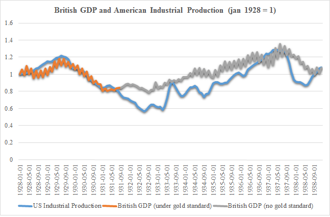
Sumner should expand on this point! To be fair, he does talk about it briefly. Not enough! A longer discussion of the British case provides him with the “extra mile” to cover the distance against competing theories. The absence of supply shocks in Britain during the Depression confirm his story that the woes of the United States during the 1930s are due to initially poor monetary policy and then poor supply-side policies. In my eyes, this is a strong confirmation of the importance of the NGDP level target argument!

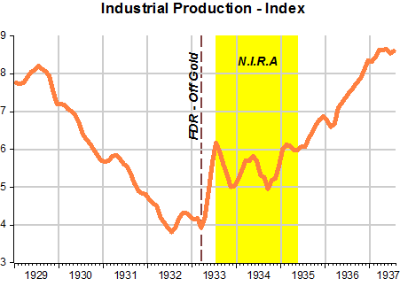
With such a point made, it is easy to imagine a reasonable counterfactual scenario of what economic growth would have been after monetary easing in 1933 in the absence of supply-side shocks. Had the United States kept very unregulated labor and product markets, it is quite reasonable to believe (given the surge seen in 1933 in the Industrial Production data) that the United States would have returned to 1929 levels. In the absence of such a prolonged economic crisis, it is hard to imagine how different the 1930s and 1940s would have been but it is hard to argue that things would have been worse.

UPDATE: From the blog Historinhas, Marcus Nunes sent me the graph below confirming the importance of the NIRA shock on eliminating all the benefit from easy money after 1933.

J Goodman (1)

Myths about the “owners of capital”

Yesterday, Steve Horwitz of Saint-Lawrence University made a small post on facebook. Basically, it was a complaint against enduring myths regarding capital owners. He pointed that “historically, the owners of capital have very often rejected free markets and asked for political privileges” and that free markets should be (solely) judged on their ability to increase the standard of living for consumers.

In essence, I share his complaint. History is a good guide on the issue. In both Canada and the United States (historically), protectionism was advanced by capital-owners who wanted to shield their capital from competition. Since both economies had abundant capital in the form of land relative to labor compared with European economies, European economies should have been the producers of labor-intensive goods such as manufactured goods. However, the “owners of capital” basically did lobby against free trade such as to protect their interests in the production of manufactured.  Indeed, these industries did expand in Canada and the US and it was good for profits (my co-author on a project regarding measuring Canadian GDP from 1870 to 1900, Michael Hinton, is coming out with a book showing Canadian productivity to be equal to American productivity in protected sectors like textiles). However, the American industries (at least in textiles) were much less productive than those found in England which had the competitive advantage in that area. Although it is a small example, it shows that the “owners” of capital are rarely about free markets and their benefits may not imply greater living standards.

However, I want to point out something important regarding capital that Horwitz fails to mention. In fact, it is the fact that his argument can be summarized in one simple sentence: the value of this capital is determined by the value of what it produces to consumers. Capital must be transformed into capital goods that are helpful in the production of consumer goods. If capital is not used to increase the production of the goods that consumers value the most, it is wasted. By definition, capital should serve consumers. If it does not, there is an incentive to reallocate capital to other areas of production to maximize profits by maximizing welfare for consumers. For example, capital-owners are very happy to lend money to individuals who invent new technologies to take more pie from an even larger pie. The main way through capital can be kept to uses that are not the most valued by consumers is through legislative coercion.

Take the case of Canada in the 19th century which we mentioned above. Capital-owners in Canada wanted to protect their investments in textiles. To do so, they had to prevent Canadian consumers from buying textiles from countries were capital was being used more efficiently to produce clothing.

Had there been free trade, Canadians would have bought more foreign cloth. Owners of capital in Canada would have had to compete with capital owners from abroad (since an increase in imports of goods means an increase in the exports of Canadian assets to foreigners which means more foreign investment in Canada) or would have had to reallocate their capital to other industries like shipping or agriculture. Canadians would have had more money in their pockets to save more money and thus increase the stock of capital to make everyone richer in the future.

I think that this was  the best way to illustrate the point made by Horwitz.

Forget income, the greatest outcome of capitalism is healthier lives!

Yesterday, James Pethokoukis of the American Enterprise Institute posted, in response to Bernie Sanders’ skepticism towards free market, that capitalism has made human “fantastically better”.

I do not disagree – quite the contrary. However, Pethokoukis makes his case by citing the fact that material quality of life has increased for everyone on earth since the early 19th century. I believe that this is not the strongest case for capitalism.  The strongest case relies on health. This is because it addresses an element that skeptics are more concerned about.

Indeed, skeptics of capitalism tend to underline that “there is more to life than material consumption”. And they are right! They merely misunderstand that the “material standard of living” is strongly related to the “stuff of life”. For them, income is of little value as an indicator. Thus, we need to look at the “quality of human life”. And what could be better than our “health”?

The substantial improvement in the material living standard of mankind has been accompanied by substantial improvements in health-related outcomes! Life expectancy, infant mortality, pregnancy-related deaths, malnutrition, risks of dying from contagious diseases, occupational fatalities, heights, the types of diseases we die from, quality of life during old age, the physical requirements of work and the risks related to famines have all gone in directions indicating substantial improvements!

My favorite is the case of height. Human stature is strongly correlated with income and other health outcomes (net nutrition, risks of disease, life expectancy, pregnancy-related variables). Thus it is an incredible indicator of the improvement in the “stuff of life”. And throughout the globe since the industrial revolution, heights have increased (not equally though).  Over at OurWorldInData.org, Max Roser shows this increase since the 1800s (in centimeters)

height-development-by-world-regions-interpolation-baten-blum-2012-0-579x500

However, the true magnitude of the increase in human heights is best seen in the data from Gregory Clark who used skeletal remains found in archaeological sites for ancient societies. The magnitude of the improvement is even clearer through this graph.

male-heights-from-skeletons-in-europe-1-2000-clark-645x403.png

The ability of “capitalism” to generate improvement in material living standards did leak into broader measures of human well-being. By far, this is the greatest outcome from capitalism.

Free Trade and Labor Market Displacement

A few days ago, I saw Noah Smith’s piece on free trade and why opening up with China may have yielded some undesirable results. In essence, his argument is that labor market adjustments have been slow. It created a small storm in the economics blogosphere. I wanted to reply earlier. I did not and I regret that. However, better late than never. So here are my three key reactions to the piece written by Smith (see his blog here).

  1. Slow labor market adjustments are not a cause of free trade: If anything, they are the results of a series of government intervention. Countries like Denmark, which may have large governments combined with fewer regulations on businesses, are very well able to adapt to free trade. The ability to start businesses is basically the ability to properly channel inputs towards more valued output. If you prevent an entrepreneur from doing just that while you open your borders to more efficient producers, it is quite obvious that free trade could be “less” beneficial. This point can be well seen in the role of states with “right to work (RTW) laws”. Although there is a debate as to whether or not RTW laws increase wages (James Sherk at Heritage says yes, the good people at the Employment Policy Institute say no and I say that both don’t get it, we should care about regionally adjusted real wage growth), it does seem that it helps industrial activity while boosting employment levels (see here too).  Unions would hinder adjustments to changes in trade patterns. In fact, its worth pointing out that of the 11 states that had RTW laws before 1948 – in only three of those states did the income share of the top 10% exceed that on the whole United States (see the data here) in 2013. While the entire country has seen an increase in income inequality, the RTW states have seen the share of all income of the top 10% increase by only 26% (1947 to 2013) compared to 42% nationwide. This suggests that RTW laws are probably helping workers adjusts to changes caused by free trade (otherwise, there would be a state-level increase in inequality). This finding seems to conform to large section of the literature on the links between RTW and inequality (here and here).  I am sure that if the Autor, Dorn and Hanson study (on which Noah Smith relies) was to be redone with attempts to control for right to work laws, the effect would be concentrated in non-RTW states. Thus, if the problem is labor laws, don’t blame free trade for the poor adjustments!
  2. Nobody said that free trade was “costless” to adapt to. I do economic history. I see cases of industries being protected for decades. Protectionism not only raise prices, but it changes relative prices between different inputs. It incites the adoption of an artificially profitable production method. It is profitable to do so, but it is by no means the most efficient approach. It was made profitable only by the artifice of regulation and duties. Once you eliminate that artifice by removing the barriers, you still have “time to build” problem and a need to change production methods. That takes time. However, governments are very good at making sure this takes more time than needed (see point 1)
  3. Trade agreements with China are not free trade agreements: this is the point I keep repeating (and the point that actually make Paul Krugman interesting), free trade agreements should normally fit on a napkin. If it takes 10,000 pages, it is free trade with 10,000 exceptions. Noah Smith should realize that he may be looking at a case of such “managed trade”.

That’s all folks!

The High Wage Economy: the Stephenson critic

A recent trend has emerged in economics. The claim is that high wages can have a dynamic positive effect on market economies.  The intuition is that high wages increase productivity because they incite management to find new techniques of production. In essence, its an argument about efficiency wages: efficiency wages increase incentives to innovate on the part of managers, they can also incite workers to acquire more human capital and work harder and more diligently.

In economic history, this claim has been taken up by scholars like Robert Allen (see his work here for the general public) who argues that the Industrial Revolution took place in England because of high wages. The high-wages of England in the 17th and 18th centuries (relative to all other areas in Europe), together with cheap energy, created an incentive for capital-intensive methods of production (i.e. the industrial revolution). In fact, a great share of the literature on the desirability of high wages for economic development has emanated from the field of economic history.

I have always been skeptical of this argument for two reasons. The first is that efficiency wages is a strange theory that relies on debatable assumptions about labor (strangely, I have been convinced of this point by Austrian scholars like Don Bellante and Pavel Ryksa). The second is that numerous scholars have advanced large criticisms of the underlying data. Robert Allen – the figurehead proponent of the high wage argument – has been constantly criticized by historians like Jane Humphries (see here) for the quality of the data and assumptions used. Allen defends himself on numerous occasions and many of his replies (mainly those on the role of family size in living standards) show that his initial case might have been too conservative (i.e. he is more “correct” than he claims).

Until a year or two ago, I was agnostic on the issue even though I was skeptical. That was until I met Judy Stephenson – a colleague at the London School of Economics. Judy did what I really like to do – dig for data (yes, I am weird like that). She went to the original sources of data used by Allen and others and she looked at what any Law-and-Economics buffs like me like to look at – transaction costs and contracting models.

She recently published her work as a working paper at the LSE and what she found is crucial! Labor was not hired directly, it was hired through contractors who charged costs on the basis of days worked. But this did not translate into wages actually paid to workers. The costs included risks and overheads for contractors. Somewhere between 20% and 30% of the daily costs were not given to workers as wages. Thus, the wage series used to claim that England (Stephenson concentrates on London though) had high wages are actually 20% to 30% below the level often reported. They are also substantially close to those in western Europe.

Thus, the high wage story for England seems weaker. This little piece of historical evidence brought about by Judy is something to think about carefully when one makes the argument that high wages are conducive to growth. Since most of the argument brought to the public was informed largely by this argument in economic history, it makes sense to be cautious when thinking about it in the future.

On the Canadian economy: the “real” problem

In Canada, the state of the economy has everyone worried. The fall in oil prices is causing the oil sector in the western provinces and in some of the Atlantic provinces to contract. As a result, everyone has the impression that Canada is sliding towards a recession and governments should act.

I disagree. My disagreement is fueled by two factors. The first is that we should never reason from a price change. The fall in the price of oil is mostly the result of increasing supply of oil. Such a price change is actually a good thing for the Canadian economy. The slowdown in economic activity is merely the result of frictions in the reallocation of resources. The second reason is that the slowdown is caused by “real factors” – policy decision affecting key regions of the Canadian economy. Any government action would worsen a situation caused by too much interference in the first place.

A fall in oil prices can indeed affect the Canadian economy. The oil produced in Canada is generally profitable when prices are relatively high (they require very capital-intensive methods of extraction and refining). An increase in the world oil supply (which is the case right now) would indeed affect the Canadian oil industry. However, Canadians win through lower oil prices – one important input has gotten cheaper. The problem is that once such a slowdown happens, resources are not reallocated without frictions. Business plans are positively affected by the lower oil prices and numerous firms are laying out new plans to expand production. Employment and output will fall in the oil industry before they will pick up in other industries. Eventually, there might even be greater output and employment because of the greater worldwide supply of oil. Right now, Canada is in-between those two situations.

My second reason for dissenting from the majority opinion is that certain regions of the Canadian economy are plagued by poor policy. To make my argument, consider a two-region (West and East) and two-industry economy (oil and manufacturing/services). In the West, the dominant industry is oil. In the East, the dominant industry is manufacturing/services.  The West economy has a more flexible market for inputs (limited regulation, freer labor market and low taxes on capital). The East economy suffers from greater rigidity in its market for inputs – high taxes, burdensome regulation and stringent labor laws.

In a way, this describes the Canadian economy. The provinces of Alberta, Saskatchewan, Manitoba and British-Columbia have been pulling the rest of the Canadian economy for the last twenty years. That’s the West. In the East, the historically poorer province of Quebec has been constantly pulling everyone behind, but less so in recent years as the province of Ontario (the most populous of Canadian provinces) began to slow down. Ontario dramatically expanded the size of its public sector, implemented important regulations and raised taxes – straight in the middle of the recession. In fact, if you exclude Ontario from the rest of Canada, you find (as Philip Cross did) that Canada’s performance is actually quite decent. So in the East, you have Quebec whose policies have not changed and you have Ontario who has adopted increasingly anti-growth policies. The East also has consistently higher taxes. The West has lower taxes. Etc.

Given the accuracy of this stylized description, imagine the effect of a shock on the western economy through a shock on its oil industry. Normally, firms in the East could adapt to lower oil prices by expanding their output in the manufacturing/services sector (thanks to cheaper inputs) while firms in the West contract their output and liberate inputs. However, in the presence of government-imposed frictions, this reallocation of resources is much harder and output has a harder time expanding in the East.

No demand-side policy can solve this problem! You could have easy money and a massive stimulus program, but if firms are discouraged from increasing output, little will happen. In Canada, the current slowdown is explained by “real factors”. Improving provincial policies would be the best channel for improving the state of the Canadian economy.

Can we use tax data to measure living standards (part 2)?

Yesterday, my post on the differences in per capita income and total income per tax unit caused some friends to be puzzled by my results. To their credit, the point can be defended that tax units are not the same as households and the number of tax units may have increased faster than population (example: a father in 1920 filled one tax unit even though his household had six members, but with more single households in the 1960s onwards the number of tax units could rise faster than population for a time).

The problems regarding the use of tax units instead of households is not new. In fact, it is one of the sticking point advanced by skeptics like Alan Reynolds (see his 2006 book) and, more recently, by Richard Burkhauser of Cornell University (see his National Tax Journal article here).

Could it be that all the differences between GDP per person and income per tax unit are caused by this problem? Not really.

There is an easy to see if the problem is real. Both measures are ratios (income over a population). Either the numerator is wrong or the denominator is wrong. Those who view tax units as the problem argue that the problem is the denominator. I do not agree since I believe that the numerator is at fault. The way to see this is simply to plot total income reported by all tax units and compare this with real GDP. What’s the result?

Even with tax-reported income being deflated with the Implicit Price Deflator (IPD) instead of the consumer price index, we end up with a difference (in 2013) of roughly 3 orders of magnitude between GDP and tax-reported income relative to the 1929 base point. Basically, GDP has increased by a factor of 14.749 since 1929 while IPD-deflated tax-reported income has only increased by a factor of 11.546.

TaxData

As a result, I do not believe that the problem is the tax unit issue. The problem seems to be that tax data is not capturing the same thing as GDP is!

Can we use tax units to measure living standards?

In the debate on inequality, I am a skeptic of how large a problem the issue is. Personally, I tend to believe that worries of inequality only increase when growth is stagnant. In fact, I also believe that there are numerous statistical biases causing us to misidentify stagnation as rising inequality. Most of the debate on inequality is plagued with statistical problems of daunting magnitudes (regional convergence in income, regional price levels, demographic changes, increasing heterogeneity of preferences, increasing heterogeneity of personal characteristics, income not being purely monetary, the role of taxes and transfers etc.)

One of them centers around the use of tax data. This has been the domain of Thomas Piketty and Emmanuel Saez. I can understand the appeal of using tax data since it is easily available and usable. Yet, is it perfect?

A year or two ago, I would have been inclined to simply say “yes” and not bother with the details. Theoretically, taxes should be an “okay” proxy for the income distribution and should follow average income even if at different levels. Yet, after reading the article of Phil Magness and Robert Murphy in the Journal of Private Enterprise I confess that I am no longer accepting anything as “granted” in the inequality debate. So, I simply decided to chart GDP per capita with the average taxable income per tax unit. Just to see what happens. Both are basically averages of the overall population, they should look pretty much the same (theoretically).  The data for the tax units is made available in the Mark W. Frank dataset based on the Piketty-Saez data (see here) and I deflated with both the CPI and the implicit price deflator available at FRED/St-Louis.

The result is the following and it shows two very different stories! Either the GDP statistics are wrong and we have average stagnation (which does not mean that there is no increase in inequality) or the taxable income data is wrong in estimating the trend of living standards and the GDP are closer to reality (which does not that there is no increase in inequality).  In the end, there is a problem to be assessed with the quality of the data used to measure inequality.

Tax Data

NGO v. NGDP: In reply to Nunes and Sumner

A week ago, I initiated a discussion on using another indicator of nominal spending instead of NGDP when the time comes to set monetary policy. My claim was that NGDP includes only final goods and as a result, it misses numerous business-to-business transactions. This means that NGDP would not be the best indicator. I propose a shift to a measure that would capture some intermediate transactions.

The result was a response by Nick Rowe (to which I did respond), Matt Rognlie, Marcus Nunes and Scott Sumner (to whom I am responding now). Nunes and Sumner are particularly skeptical of my claim. I am providing a first response here (and I am attempting to expand it for a working paper).

The case against NGDP

GDP has important shortcomings. First of all, thanks to the work of Prescott and McGrattan (2012 : 115-154), we know that a sizable part of capital goods acquisition fails to be included inside GDP. That sizable part is “intangible capital” which Prescott and McGrattan define as the “accumulated know-how from investing in research and development, brands, and organizations which is the most part expensed rather than capitalized” (p.116).  Yet, investments in research and development are – in pure theoretical terms – like the acquisition of capital goods. However, national accounts exclude those. Once they’re included in papers like those of Prescott and McGrattan and those of Corrado, Hulten and Sichel (2009), increases in productivity were faster prior to 2008 and that the collapse after 2008 was much more pronounced.  In addition, this form of capital is increasing much faster than tangible so that its share of the total capital stock increases. Thus, the error of not capturing this form of capital good investment is actually growing over time causing us to miss both the level and the trend.

A second shortcoming of importance is the role of time in production. Now, just the utterance of these words makes me sound like an Austrian. Yet, this point is very neoclassical since it relies on the time to build approach. In the time-to-build model of the real business cycle approach, production occurs over many periods. Thus changes in monetary policy may have some persistence.  The time-to-build model proposes that firms undertake long projects and consume more inputs. In terms of overall transactions, this will mean more and more business to business (B2B) transactions.  Hence if an easy monetary policy is inciting individuals to expand their number of projects that have more distant maturities, then a focus on GDP won’t capture the distortionary effects of that policy through. Similarly, if monetary policy tightens (either directly as a fall of the money supply or through an uncompensated change in velocity), the drop in economic activity as projects are closed down will not equally well captured. While this point was initially advanced by Kyland and Prescott (1982), some Austrians economists have taken up the issue (Montgomery 1995a; 1995b; 2006; Wainhouse 1984; Mulligan 2010), several neoclassicals have also taken it up (Kühn 2007; Kalouptsidi 2014; Kyland, Rupert, Sustek, 2014).

Why shift to another measure

My contention is that NGO (Nominal Gross Output) allows us to solve a part of that problem. First of all, NGO is more likely to capture a large share of the intangible capital part since, as a statistic, it does not concern itself with double counting. Hence, most of the intangible capital expenses are captured. Secondly, it also captures the time-to-build problem by virtue of capturing inputs being reallocated to the production of projects with longer maturities.

Thus, NGO is a better option because it it tries to capture the structure of production. The intangible capital problem and the time to build problem are both problems of intermediate goods. By capturing those, we get a better approximate idea of the demand for money.

Let me argue my case based on the Yeager-esque assumption that any monetary disequilibrium is a discrepancy between actual and desired money holdings at a given price level. Let me also state the importance of the Cantillon effects whereby the point of entry of money is important.

If an injection of money is made through a given sector that leads him to expand his output, the reliability of NGDP will be best if the entry-point predominantly affects final goods industry. If it enters through a sector which desires to spend more on intangible investments or undertake long-term projects, then the effects of that change will not appear as they will merely go unmeasured. They will nonetheless exist. Eventually firms will realize that they took credit for these projects for which the increased output did not meet any demand. The result is that they have to contract their output by a sizable margin. In that case, they will abandon those activities (imagine unfinished skyscrapers or jettisoned research projects).

In such situations, GO (or even a wider measure of gross domestic expenditures) are superior to GDP. And in cases where the effects would start in final-goods industry, then they have the same efficiency as GO (or the wider measure of gross domestic expenditures.

The empirical case

The recurring criticism in most posts is that NGO is volatile over the period when the data is available (2005Q1-today). True, the average growth rate of NGO is the same as NGDP over the same period, but the standard deviation is nearly twice that of NGDP. However if you exclude the initial shock of the recession, the standard deviations converge. In a way, all the difference in volatility between the two series is driven by the shock of the recession. Another way to see it is to recompute two graphs. One is an imitation of the graphs by Nunes where NGDP growth in period T is compared with growth in the period T minus 1, but we add NGO. The second is the ratio of NGO to NGDP.

As one can see from the first figure, NGO and NGDP show the same relation except for a cluster of points at the bottom for NGO. All of those lower points are related to the drop from the initial recession. All concentrated at the bottom. This suggests that the recession had a much deeper effect than otherwise believed. The second graph allows us to see it.

Nunes

The ratio of NGO to NGDP shows that the two evolved roughly the same way over the period before the recession. However, when the recession hit, the drop was more important and the ratio never recovered!  This suggest a much deeper deviation from the long-term trend of nominal spending which is not seen at the final level but would be seen rather in the undertaking of long-term projects and the formation of intangible capital (the areas that NGDP cannot easily capture).

Ratio.png

The case for NGO over NGDP is solid. It does not alter the validity of the case for nominal spending stability. However since the case for nominal spending stability hinges on total transactions of inputs and outputs more than it does on the final goods sold, NGO is a better option.


Quick comment in response to Rognlie 
In his reply to Nick Rowe, Matt Rognlie states that the more important fall of NGO is explained by changes in relative prices. Although his transformation shows this, the BEA disagrees. Here is the explanation provided by the BEA:
For example, value added for durable-goods manufacturing dropped 15 percent in 2009, while gross output dropped 19 percent.  The decline in gross output is much more pronounced than the decline in value added because it includes each of the successive declines in the intermediate inputs supply chain required to manufacture the durable goods.


Why farms die and should die


In Canada, I have the frustrating habit of criticizing government support to the agricultural sector especially entry-barriers in the form of production quotas. Most of those policies are regressive in the sense that they reallocate income from the poorest to the richest. In fact, their entire aim is to artificially increase the income of farmers (especially dairy and poultry farmers) at the expense of the rest of the population. However, when lobbyists for these subsidies come out in public, they do so under different disguises. Their favorite? Farms are dying.

In each radio debate where that boogeyman is raised, I reply that “yes, they are dying and its a good thing”. If we can feed more and more people with less and less farmers using less and less land, that’s a good thing. In fact, it’s the greatest thing that happened in economic history. Less two centuries ago, 90% of the workers in some western economies were involved in agricultural activities. Today, that proportion has fallen to less than 1.5%. Thousands of farms disappeared, we liberated millions of acres of land to return to their natural state and in the process, we became rich and well-fed!

In testimony of this fact, which is my favorite economic history fact, I decided to recompute a graph by Mark Perry of the American Enterprise Institute but I added the GDP per capita figures for the same period (1790 to 2013).

GDPagriculture

Yes, let the farms die. Let the most productive stay in the fields and let them feed humanity while the others become engineers, doctors, teachers, businessmen, welders, carpenters or whatever trade they are best at!

Basic income: a debate where demand magically disappears!

For a few months now, the case for the basic income has resurged (I thought it died with Milton Friedman in 2006, if not earlier). In the wake of this debate, I have been stunned by the level of disconnect between the pundits and what the outcome of the few experiments of basic income have been. The most egregious illustration of this disconnect is the case of the work disincentive.

To be clear, most of the studies find a minor effect on labor supply overall which in itself does not seem dramatic (see Robert Moffitt’s work here). Yet, this is a incomplete way to reflect on the equilibrium effect of a massive reform that would be a basic income.

Personally, I think that there is a good reason to believe that the labor supply reaction would be limited. At present, many tax systems have”bubbles” of increasing marginal tax rates. In some countries like Canada, the phasing out of tax credits for children actually mean that the effective marginal tax rate increases as income increases from the low 20,000$ to the mid 40,000$. As a result, a basic income would flatten the marginal tax rate for those whose labor supply curve is not likely to bend backward. In such a situation, labor supply could actually increase!

Yet, even if that point was wrong, labor supply could shift but without any changes in total labor provided. Under most basic income proposals, tax rates are dropped significantly as a result of a reduced bureaucracy and of a unified tax base (i.e. the elimination of tax credits). In such a situation, marginal tax rates are also lowered. This means greater incentives to invest (save) and acquire human capital. This will affect the demand for labor!

A paper in the Journal of Socio-Economics by  Karl Widerquist makes this crucial point. None of the experiments actually could estimate the demand-side reaction of the market. Obviously, a very inelastic labor demand would mean very little change in hours worked and the reverse if it was very elastic. But what happens if the demand curve shifts? Widerquist does not elaborate on shifts of the demand curve, but they could easily occur if a basic income consolidates all transfers (in kind and conditional monetary) allows a reduction in overall spending and thus the tax take needed to fund activities. In that case, demand for labor would shift to the right. A paper on the health effects of MINCOME in Manitoba (Canada) shows that improvement in health outcomes are cheaply attained through basic income which would entail substantial health care expenditures reduction.

I have surveyed the articles compiled by Widerquist and added those who have emerged since. None consider the possibility of a shift of the demand curve. Even libertarian scholars like Matt Zwolinski (who has been making the case forcibly for a basic income for sometime now) have not made this rebuttal point!

Yet, the case is relatively straightforward: current transfers are inefficient, basic income is more efficient at obtaining each unit of poverty reduction, basic income requires lower taxes, basic income means lower marginal tax rates, lower marginal tax rates mean more demand for investment and labor and thus more long-term growth and a counter-balance to any supply-side effect.

I hope that the Bleeding Heart Libertarians will take notice of this crucial point in favor of their argument!

Women and secular stagnation

As an economic historian, I’ve always had a hard time with the idea of secular stagnation. After all, one decade of slow growth is merely a blip on the twelve millenniums of economic history (I am not that interested with the pre-Neolithic history, but there is some great work to be found in archaeology journals). Hence, Robert Gordon’s arguments fall short on me.

That was until I was sparked to react to a comment by Emily Skarbek at Econlib. Overall, she is skeptical of Gordon’s claims of secular stagnation. But not for the same reasons. She claims that there are many improvements in welfare that we are not capturing through national income accounts. This is basically the same point as the one made by the great Joel Mokyr (the gold standard of economic historians).

It is true that national accounts have some large conceptual problems regarding measuring output when there are massive technological changes. Yet, all these problems don’t go in the same direction. More precisely, they don’t all lead to underestimation of growth.

My favorite example of one that leads us to overestimate growth is the one I keep giving my macroeconomics students at HEC Montreal. Assume an economy with a labor-force participation rate of 50%. Basically, only males work. All women stay at home for household chores and childcare. In that case, all measured output is male-produced output. Since national accounts don’t consider household production, all the output of women in the households of this scenario is non-existent.

Now assume a technological change causing a shift of 10% of women to the workforce at the same wage rate as men. That boosts labor participation rate to 55% and output by 5%. However, that would largely overestimate growth caused by this shift. After all, when my grandmothers were raising my parents, they were producing something. It was not worthless output. Obviously, if my grandmothers went to work, there was some net added value, but not as much as 5%. However, according to national account, the net increase in GDP is … 5%.

Obviously wrong right? Now, think of the economic history of the last 100 years. Progressively, female labor-force participation increased as marriages were delayed and family sizes were reduced. Unmarried women stayed on the market longer. Then, the introduction of new household technologies allowed some married women to join the labor force more actively. Progressively, women accumulated more human capital and became more active in the labor force. So much that in many western countries, both genders have equal labor-force participation rates.

As they shifted from household production to market production, we considered that everything they did was a net added value. We never subtracted the value of what was produced before. Don’t get me wrong, I am happy that women work instead of toiling inside a household to handwash dirty clothes. Yet, it would be both statistically incorrect and morally insulting to say that what women did in the household had no value whatsoever. 

The role of household production in reducing the quality of growth estimates goes back to the 1870s! A 1996 article in Feminist Economics (which I use a lot in my own national account sections of macroeconomics classes) shows the following changes in growth rates when we account for the value of household production. Instead of increasing to 1910 and then falling to 1930, growth in the United States falls to 1930. While the growth rates remain appreciable, they nonetheless indicate a massively different interpretation of American economic history.

SecularStagnation


Sadly, I do not possess a continuation of such estimates to later points in time for the United States. I know there is an article by the brilliant Valerie Ramey in the Journal of Economic History, but I am not sure how to compute this to reflect changes in overall output. I intend to try to find them for a short piece I want to submit later in 2016. Yet, I do have estimates for my home country of Canada. Combining a 1979 paper in the Review of Income and Wealth with a working paper from Statistics Canada, it seems that the value of household production falls from 45% of GNP in 1961 to 33% in 1998. When we adjust GDP per capita to consider the changes in household work in Canada, the growth path remains positive, but it is less impressive.

SEcularStagnation2

I am not saying that Gordon is right to say that growth is over. I am saying that the accounting problems don’t all go in the direction of invalidating him. In fact, if my point is correct, proper corrections would reduce growth rates dramatically for the period of 1945 to 1975 and less so for the period that followed. This may indicate that “slow growth” was with us for most of the post-war era. That’s why I reacted to the blog post of Skarbek.

It also allows me to say the thing that is the best buzz-kill for economics students: national accounting matters!

Of Uber, cab drivers and compensation

What a title for a blog post right? Where am I going with this? A few days ago, I debated a few of my academic colleagues who tend towards libertarianism in the predominantly left-leaning province of Quebec. The topic? How the rise of Uber is killing the taxi cartel? I authored a paper on ride-sharing a year ago and I cannot be more enthusiastic towards such technologies that are allowing consumers much more choices at lower prices than with the taxi cartel. Thus, we were all in agreement. The point of contention appeared when the topic of compensation was raised. I favor partial compensation of the owners of taxi licences. Instantly, I was cast in the minority position and branded as a statist. A debate ensued and I made the case that it was not acceptable to right a wrong by committing another wrong (how Christian of me).

First, let me lay out some facts first and some assumptions

  1. A taxi licence restricting competition is a subsidy. But it is a strange type of subsidy that occurs through a redistribution of property rights (limiting the right to use one’s own car to carry individuals in exchange for payment to those who buy the transferable right to do so). Unlike cash subsidies, quotas, trade barriers and tax credits, it is the only form of income transfer that exists that is a property. You can abolish any cash subsidy, tariff, quota, tax, tax credits or legal monopoly without having to compensate since no one has property of such things. That is the source of the odd nature of the taxi licence – a subsidy with a property deed.
  2. The two benefits from these licences occur through limiting competition and thus allowing higher prices/quality ratios and through higher asset value (the permit’s value). The extent of those benefits depends on the extent of the curtailment of the liberties of other to compete. The more restrictive the policy, the greater the redistribution from consumers to producers in the long-run.
  3. However, new drivers have to pay a high price and they must have some time to recoup the acquisition of the asset. Their recovery will take some time as they also hike prices and lower quality.

So, if you want to abolish a taxi licensing scheme, is it acceptable not to compensate? According to my colleagues, yes it is. Since the benefits of higher prices were so considerable to those drivers (at the expense of consumers), compensation is not necessary.

Yet, the drivers do own property don’t they? The licence is worth many thousands of dollars, basically the value of a small house. Many drivers rely on this asset for their retirement. Now, let me make another presumption which is crucial to this discussion: the change is caused by legal changes, not technological changes.

I believe that, in the presence of the technological change, there is no case for compensation. Nobody would compensate telecoms companies for the rise of Skype since it is a process of entrepreneurship. However, the case is different if a government decides to abolish the licences. So here, my entire reasoning for compensation is contingent to a case where the state abolishes the licences, not a situation where technologies render the licences worthless like the car killed the street horses.

Clearly, it was unjust for consumers to deal with a cartel that gouged them and which was legally sanctioned to do so. But can you right an injustice by committing another injustice (the de facto dispossession of an asset)? Normatively speaking, I simply believe that using the monopoly of violence of the state to right the abuses caused by past uses of the monopoly of violence of the state is not that productive. Why? Because I have this assumption lodged firmly in my head as a result of my training in public choice theory: rent-seeking matters.

Rent-seekers will always exist. They are the social-science equivalent of gravity in physics. You just have to deal with their existence. Rent-seekers are basically political entrepreneurs who have very concentrated benefits from applying policies whose costs are not that obvious or that important for a large population. These political entrepreneurs are very alert to opportunities and they will seize them. Sometimes, they discover that their preferred course of action leads to resistance. They will automatically shift gear and find another way to obtain an unearned reward thanks to the complicity of those they bargain with (politicians and bureaucrats). Their rhetoric will change, their narratives will change, their arguments will evolve, but at the core, they will continue to rent-seek. True, you can conceive constitutional rules that limit rent-seeking (I am a big fan of that). However, one way or another, it will remain and some will find ways to connive with politicians and bureaucrats to obtain undue rewards. And even if there was such a utopia free of rent-seekers (I just won’t buy that for a dollar) where a constitution would ban their activities or even a stateless utopia (again, I am not buying it), is it acceptable to justify all means possible to reach such a destination?

What if associations of cab drivers lobby for special tax discounts on gasoline since they provide a public service? What if they lobby for stricter security checks on drivers (needless security checks) which end up having the same effects? What if they convinced regulators that only certain types of vehicles (less than 5 years old for example) should be allowed to operate? What if they mandated association with a dispatcher to better avoid traffic jams? How could a politician oppose special tax treatment for drivers, better security for consumers or all these other bogus motives? In the end, they will find a way to rent-seek. However, by dispossessing them of an asset worth many hundred of thousands of dollars, you are basically creating the certainty that they will aggressively rent-seek to recuperate their losses. Thus, you don’t end up breaking a vicious policy cycle, you end up encouraging its continuation in stranger, hidden and subtle manners whose perniciousness continues equally.

Hence my case that you can’t right a wrong by committing a wrong. Respect the rule of law, liberalize the market and compensate and attempt to rewrite constitutions to prevent arbitrary redistribution of property rights.

Malthusian pressures (as outcome of rent-seeking)

Nearly a week ago, I intervened in a debate between Anton Howes of King’s College London whose work I have been secretly following  (I say “secretly” because as an alumnus of the London School of Economics, I am not allowed to show respect for someone of King’s College) and Pseudoerasmus (whose identity is unknown but whose posts are always very erudite and of high quality – let’s hope I did not just write that about an alumnus of King’s College). Both bloggers are heavily involved in my first field of interest – economic history.

The debate concerned the “Smithian” counter-effect to “Malthusian pressures”. The latter concept refers to the idea that, absent technological innovation,  population growth will lead to declining per capita as a result of marginally declining returns. The former refers to the advantages of larger populations: economies of scale, more scope for specialization and market integration thanks to density. Now, let me state outright that I think people misunderstand Malthusian pressures and the Smithian counter-effect.

My point of is that both the “Smithian counter-effect” and “Malthusian pressures” are merely symptoms of rent-seeking or coordination failures. In the presence of strong rent-seeking by actors seeking to reduce competition, the Smithian counter-effect wavers and Malthus has the upper hand. Either through de-specialization, thinner of markets, shifting to labor-intensive technologies, market disintegration and lower economies of scale, rent-seeking diminishes the A in a classical Cobb-Douglas function of Total Factor Productivity (Y=AKL). This insight is derived from my reading of the article by Lewis Davis in the Journal of Economic Behavior and Organization which contends that “scale effects” (another name for a slight variant of the “Smithian counter-effect) are determined by transaction costs which are in turn determined by institutions. If institutions tend to favor rent-seeking, they will increase the likelihood of coordination failure. It is only then that coordination failures will lead to “Malthusian pressures” with little “Smithian counter-effect”. Institutions whose rules discourage rent-seeking will allow markets to better coordinate resource use so as to maximize the strength of the “Smithian counter-effect” while minimizing the dismal Malthusian pressures.

In essence, I don’t see the issue as one of demography, but as one of institutions, public choice and governance. I am not alone in seeing it this way (Julian Simon, Jane Jacobs and Ester Boserup have documented this well before I did). Why the divergence?

This is because many individuals misunderstand what “Malthusian pressures” are. In an article I published in the Journal of Population Research, me and Vadim Kufenko summarize the Malthusian model as a “general equilibrium model”. In the long run, there is an equilibrium level of population with a given technological setting. In short-run, however, population responds to variation in real wages. Higher real wages from a “temporary” positive real shock will lead to more babies. However, once the shock fades, population will adapt through two checks: the preventive check and the positive check. The preventive check refers to households delaying family formation. This may be expressed through later marriage ages, planned sexual activities, contraception, longer stays in the parental household and greater spacing between births. The positive check refers to the impact of mortality increasing to force the population back to equilibrium level. These checks return to the long-term equilibrium. Hence, when people think of “Malthusian pressures”, they think of population growth continuing unchecked with scarce ressources. But the “Malthusian model” is basically a general equilibrium model of population under fixed technology. In that model, there are no pressures since the equilibrium rates of births and deaths are constant (at equilibrium).

However, with my viewpoint, the equilibrium levels move frequently as a result of institutional regimes. They determine the level of deaths and births. “Poor” institutions will lead to more frequent coordination failures which may cause, for a time, population to be above equilibrium – forcing an adjustment. “Poor” institutions would also lead to an inability to respond to a change in constraints (i.e. the immediate environment) by being rigid or stuck with path-depedency problems which would also imply the need for an adjustment.  “Good” institutions will allow “the Smithian counter-effect” to intervene through arbitrage across markets to smooth the effect of local shocks, a greater scope for specialization etc.

My best case for illustration is a working paper I have with Vadim Kufenko (University of Hohenheim) and Alex Arsenault Morin (HEC Montréal) where we argue that population pressures as exhibited by the very high levels of infant mortality rates in mid-19th century Quebec were the result of institutional regimes. The system of land tenure for the vast majority of the population of Quebec was “seigneurial” and implied numerous regressive transfers and monopoly rights for landlords. This system was also associated with numerous restrictions on mobility which limited the ability of peasants to defect and move. However, a minority of the population (but a growing one) lived under a different institution which did not impose such restrictions, duties and monopolies. In these areas, infant mortality was considerably lower. We find that, adjusting for land quality and other factors, infant mortality was lower in these areas for most age groups. Hence, we argued that what was long considered as “Malthusian pressures” were in fact “institutional pressures”.

Hence, when I hear people saying that there are problems linked to “growing population”, I hear “because institutions make this a problem” (i.e. rent seeking).

Was Murphy Foolish to Take Caplan’s Bet?

A few days ago, Bryan Caplan posted on his bet with Robert Murphy regarding inflation. Murphy predicted 10% inflation. He lost … big time. However, was he crazy to make that bet?  In other words, what could explain Caplan’s victory?

Murphy was not alone in predicting this, I distinctly remember a podcast between Russ Roberts and Joshua Angrist on this where Roberts tells Angrist he expected high inflation back in 2008. Their claims were not indefensible. Central banks were engaging in quantitative easing and there was an important increase of the state money supply. There was a case to be made that inflation could surge.

It did not. Why?

In a tweet, Caplan tells me that monetary transmission channels are much more complex than they used to be and that the TIPS market knew this. Although I agree with both these points, it does not really explain why it did not materialize. I am going to propose two possibilities of which I am not fully convinced myself but whose possibility I cannot dismiss out of hand.

Imagine an AS-AD graph. If Murphy had been right, we should have seen aggregate demand stimulated to a point well above that of long-run equilibrium. Yet, its hard to see how quantitative easing did not somehow stimulate aggregate demand.  Now, if aggregate demand was falling and that quantitative easing merely prevented it from falling, this is what would prove Murphy wrong. However, all of this assumes no movement of supply curves.

While AD falls and before monetary policy kicks in, imagine that policies are adopted that reduce the potential for growth and productivity improvement. In a way, this would be the argument brought forward by people like Casey Mulligan in work on labor supply and the “redistribution recession” and Edward Prescott and Ellen McGrattan who argue that, once you account for intangible capital, the real business cycle model is still in play (there was a TFP shock somehow). This case would mean that as AD fell, AS fell with it. I would find it hard to imagine that AS shifted left faster than AD. However, a relatively smaller fall of AS would lead to a strong recession without much deflation (which is what we have seen in this recession). Personally, I think there is some evidence for that. After all, we keep reducing the estimate for potential GDP everywhere while the policy uncertainty index proposed by Baker, Bloom and Davids shows a level change around 2008.  Furthermore, there has been a wave – in my opinion of very harmful regulations – which would have created a maze of administrative costs to deal with (and whose burden is heavy according to Dawson and Seater in the Journal of Economic Growth). That could be one possibility that would explain why Murphy lost.

download

There is a second possibility worth considering (and one which I find more appealing): the role of financial regulations. Now, I may have been trained mostly by Real Business Cycle guys, but I do have a strong monetarist bent. I have always been convinced by the arguments of Steve Hanke and Tim Congdon (I especially link Congdon) and others that what you should care about is not M1 or M2, but “broad money”. As Hanke keeps pointing out, only a share of everything that we could qualify broadly as “money” is actually “state money”. The rest is “private money”. If a wave of financial regulations discourages banks to lend or incite them to keep greater reserves, this would be the equivalent of a drop of the money multiplier. If those regulations are enacted at the same time as monetary authorities are trying to offset a fall in aggregate demand, then the result depends on the relative impact of the regulations. The data for “broad money” (Hanke defines it as M4) shows convincingly that this is a potent contender. In that case, Murphy’s only error would have been to assume that the Federal Reserve’s policy took place with everything else being equal (which was not the case since everything seemed to be moving in confusing directions).

globr-asia-nov-2014-1bg

In the end, I think all of these explanations have value (a real shock, a banking regulation shock, an aggregate demand shock). In 25 years when economic historians such as myself will study the “Great Recession”, they will be forced to do like they do with Great Depression: tell a multifaceted story of intermingled causes and counter-effects for which no single statistical test can be designed. When cases like these emerge, it’s hard to tell what is happening and those who are willing to bet are daredevils.

P.S. I have seen the blog posts by Scott Sumner and Marcus Nunes regarding my NGO /NGDP claims. They make very valid points and I want to take decent time to address them, especially since I am using the blogging conversation as a tool to shape a working paper.